Recursive macroeconomic theory, Thomas Sargent 2nd Ed - Chapter 26 pot
Bạn đang xem bản rút gọn của tài liệu. Xem và tải ngay bản đầy đủ của tài liệu tại đây (415.95 KB, 57 trang )
Chapter 26
Equilibrium Search and Matching
26.1. Introduction
This chapter presents various equilibrium models of search and matching. We
describe (1) Lucas and Prescott’s version of an island model, (2) some matching
models in the style of Mortensen, Pissarides, and Diamond, and (3) a search
model of money along the lines of Kiyotaki and Wright.
Chapter 5 studied the optimization problem of a single unemployed agent
who searched for a job by drawing from an exogenous wage offer distribution.
We now turn to a model with a continuum of agents who interact across a
large number of spatially separated labor markets. Phelps (1970, introductory
chapter) describes such an “island economy,” and a formal framework is analyzed
by Lucas and Prescott (1974). The agents on an island can choose to work at the
market-clearing wage in their own labor market, or seek their fortune by moving
to another island and its labor market. In an equilibrium, agents tend to move
to islands that experience good productivity shocks, while an island with bad
productivity may see some of its labor force depart. Frictional unemployment
arises because moves between labor markets take time.
Another approach to model unemployment is the matching framework de-
scribed by Diamond (1982), Mortensen (1982), and Pissarides (1990). These
models postulate the existence of a matching function that maps measures of
unemployment and vacancies into a measure of matches. A match pairs a worker
and a firm who then have to bargain about how to share the “match surplus,”
that is, the value that will be lost if the two parties cannot agree and break the
match. In contrast to the island model with price-taking behavior and no exter-
nalities, the decentralized outcome in the matching framework is in general not
efficient. Unless parameter values satisfy a knife-edge restriction, there will ei-
ther be too many or too few vacancies posted in an equilibrium. The efficiency
problem is further exacerbated if it is assumed that heterogeneous jobs must
be created via a single matching function. This assumption creates a tension
between getting an efficient mix of jobs and an efficient total supply of jobs.
– 935 –
936 Equilibrium Search and Matching
As a reference point to models with search and matching frictions, we also
study a frictionless aggregate labor market but assume that labor is indivisible.
For example, agents are constrained to work either full time or not at all. This
kind of assumption has been used in the real business cycle literature to gener-
ate unemployment. If markets for contingent claims exist, Hansen (1985) and
Rogerson (1988) show that employment lotteries can be welfare enhancing and
that they imply that only a fraction of agents will be employed in an equilib-
rium. Using this model and the other two frameworks that we have mentioned,
we analyze how layoff taxes affect an economy’s employment level. The different
models yield very different conclusions, shedding further light on the economic
forces at work in the various frameworks.
To illustrate another application of search and matching, we study Kiyotaki
and Wright’s (1993) search model of money. Agents who differ with respect to
their taste for different goods meet pairwise and at random. In this model, fiat
money can potentially ameliorate the problem of “double coincidence of wants.”
26.2. An island model
The model here is a simplified version of Lucas and Prescott’s (1974) “island
economy.” There is a continuum of agents populating a large number of spatially
separated labor markets. Each island is endowed with an aggregate production
function θf(n)wheren is the island’s employment level and θ>0isan
idiosyncratic productivity shock. The production function satisfies
f
> 0,f
< 0, and lim
n→0
f
(n)=∞. (26.2.1)
The productivity shock takes on m possible values, θ
1
<θ
2
< < θ
m
,and
the shock is governed by strictly positive transition probabilities, π(θ, θ
) > 0.
That is, an island with a current productivity shock of θ faces a probability
π(θ, θ
) that its next period’s shock is θ
. The productivity shock is persis-
tent in the sense that the cumulative distribution function, Prob (θ
≤ θ
k
|θ)=
k
i=1
π(θ, θ
i
), is a decreasing function of θ.
At the beginning of a period, agents are distributed in some way over the
islands. After observing the productivity shock, the agents decide whether or not
to move to another island. A mover forgoes his labor earnings in the period of
the move, while he can choose the destination with complete information about
An island model 937
current conditions on all islands. An agent’s decision to work or to move is taken
so as to maximize the expected present value of his earnings stream. Wages are
determined competitively, so that each island’s labor market clears with a wage
rate equal to the marginal product of labor. We will study stationary equilibria.
26.2.1. A single market (island)
The state of a single market is given by its productivity level θ and its beginning-
of-period labor force x. In an equilibrium, there will be functions mapping
this state into an employment level, n(θ, x), and a wage rate, w(θ, x). These
functions must satisfy the market-clearing condition
w(θ, x)=θf
n(θ, x)
and the labor supply constraint
n(θ, x) ≤ x.
Let v(θ, x) be the value of the optimization problem for an agent finding
himself in market (θ,x) at the beginning of a period. Let v
u
be the expected
value obtained next period by an agent leaving the market; a value to be deter-
mined by conditions in the aggregate economy. The value now associated with
leaving the market is then βv
u
. The Bellman equation can then be written as
v(θ, x)=max
βv
u
,w(θ, x)+βE [v(θ
,x
)|θ, x]
, (26.2.2)
where the conditional expectation refers to the evolution of θ
and x
if the
agent remains in the same market.
The value function v(θ, x)isequaltoβv
u
whenever there are any agents
leaving the market. It is instructive to examine the opposite situation when
no one leaves the market. This means that the current employment level is
n(θ, x)=x and the wage rate becomes w(θ, x)=θf
(x). Concerning the
continuation value for next period, βE [v(θ
,x
)|θ, x], there are two possibilities:
Case i. All agents remain, and some additional agents arrive next period. The
arrival of new agents corresponds to a continuation value of βv
u
in the market.
Any value less than βv
u
would not attract any new agents, and a value higher
938 Equilibrium Search and Matching
than βv
u
would be driven down by a larger inflow of new agents. It follows that
the current value function in equation (26.2.2) can under these circumstances
be written as
v(θ, x)=θf
(x)+βv
u
.
Case ii. All agents remain, and no additional agents arrive next period. In this
case x
= x, and the lack of new arrivals implies that the market’s continuation
value is less than or equal to βv
u
. The current value function becomes
v(θ, x)=θf
(x)+βE [v(θ
,x)|θ] ≤ θf
(x)+βv
u
.
After putting both of these cases together, we can rewrite the value function
in equation (26.2.2) as follows,
v(θ, x)=max
βv
u
,θf
(x)+min
βv
u
,βE[v(θ
,x)|θ]
. (26.2.3)
Given a value for v
u
, this is a well-behaved functional equation with a unique
solution v(θ, x). The value function is nondecreasing in θ and nonincreasing in
x.
On the basis of agents’ optimization behavior, we can study the evolution of
the island’s labor force. There are three possible cases:
Case 1. Some agents leave the market. An implication is that no additional
workers will arrive next period when the beginning-of-period labor force will be
equal to the current employment level, x
= n. The current employment level,
equal to x
, can then be computed from the condition that agents remaining in
the market receive the same utility as the movers, given by βv
u
,
θf
(x
)+βE [v(θ
,x
)|θ]=βv
u
. (26.2.4)
This equation implicitly defines x
+
(θ) such that x
= x
+
(θ)ifx ≥ x
+
(θ).
Case 2. All agents remain in the market, and some additional workers arrive next
period. The arriving workers must expect to attain the value v
u
, as discussed
in case i. That is, next period’s labor force x
must be such that
E [v(θ
,x
)|θ]=v
u
. (26.2.5)
This equation implicitly defines x
−
(θ) such that x
= x
−
(θ)ifx ≤ x
−
(θ). It
can be seen that x
−
(θ) <x
+
(θ).
An island model 939
Case 3. All agents remain in the market, and no additional workers arrive next
period. This situation was discussed in case ii. It follows here that x
= x if
x
−
(θ) <x<x
+
(θ).
26.2.2. The aggregate economy
Theprevioussectionassumedanexogenousvaluetosearch,v
u
. This assump-
tion will be maintained in the first part of this section on the aggregate economy.
The approach amounts to assuming a perfectly elastic outside labor supply with
reservation utility v
u
. We end the section by showing how to endogenize the
value to search in the face of a given inelastic aggregate labor supply.
Define a set X of possible labor forces in a market as follows.
X ≡
x ∈
x
−
(θ
i
) ,x
+
(θ
i
)
m
i=1
: x
+
(θ
1
) ≤ x ≤ x
−
(θ
m
)
,
if x
+
(θ
1
) ≤ x
−
(θ
m
);
x ∈ [x
−
(θ
m
) ,x
+
(θ
1
)]
, otherwise;
The set X is the ergodic set of labor forces in a stationary equilibrium. This can
be seen by considering a single market with an initial labor force x. Suppose
that x>x
+
(θ
1
); the market will then eventually experience the least advanta-
geous productivity shock with a next period’s labor force of x
+
(θ
1
). Thereafter,
the island can at most attract a labor force x
−
(θ
m
) associated with the most
advantageous productivity shock. Analogously, if the market’s initial labor force
is x<x
−
(θ
m
), it will eventually have a labor force of x
−
(θ
m
) after experienc-
ing the most advantageous productivity shock. Its labor force will thereafter
never fall below x
+
(θ
1
) which is the next period’s labor force of a market expe-
riencing the least advantageous shock [given a current labor force greater than
or equal to x
+
(θ
1
)]. Finally, in the case that x
+
(θ
1
) >x
−
(θ
m
), any initial
distribution of workers such that each island’s labor force belongs to the closed
interval [x
−
(θ
m
) ,x
+
(θ
1
)] can constitute a stationary equilibrium. This would
be a parameterization of the model where agents do not find it worthwhile to
relocate in response to productivity shocks.
940 Equilibrium Search and Matching
In a stationary equilibrium, a market’s transition probabilities among states
(θ, x)aregivenby
Γ(θ
,x
|θ, x)=π(θ, θ
) · I
x
= x
+
(θ)andx ≥ x
+
(θ)
or
x
= x
−
(θ)andx ≤ x
−
(θ)
or
x
= x and x
−
(θ) <x<x
+
(θ)
,
for x, x
∈ X and all θ, θ
;
where I(·) is the indicator function that takes on the value 1 if any of its
arguments are true and 0 otherwise. These transition probabilities define an
operator P on distribution functions Ψ
t
(θ, x; v
u
) as follows: Suppose that at
a point in time, the distribution of productivity shocks and labor forces across
markets is given by Ψ
t
(θ, x; v
u
); then the next period’s distribution is
Ψ
t+1
(θ
,x
; v
u
)=P Ψ
t
(θ
,x
; v
u
)
=
x∈X
θ
Γ(θ
,x
|θ, x)Ψ
t
(θ, x; v
u
) .
Except for the case when the stationary equilibrium involves no reallocation of
labor, the described process has a unique stationary distribution, Ψ(θ, x; v
u
).
Using the stationary distribution Ψ(θ, x; v
u
), we can compute the economy’s
average labor force per market,
¯x(v
u
)=
x∈X
θ
x Ψ(θ, x; v
u
) ,
where the argument v
u
makes explicit that the construction of a stationary
equilibrium rests on the maintained assumption that the value to search is ex-
ogenously given by v
u
. The economy’s equilibrium labor force ¯x varies neg-
atively with v
u
. In a stationary equilibrium with labor movements, a higher
value to search is only consistent with higher wage rates, which in turn require
higher marginal products of labor, that is, a smaller labor force on the islands.
From an economy-wide viewpoint, it is the size of the labor force that is
fixed, let’s say ˆx, and the value to search that adjusts to clear the markets. To
find a stationary equilibrium for a particular ˆx, we trace out the schedule ¯x(v
u
)
for different values of v
u
. The equilibrium pair (ˆx, v
u
) can then be read off at
the intersection ¯x(v
u
)=ˆx, as illustrated in Figure 26.2.1.
A matching model 941
x(v )
u
-
x
-
v
u
x
^
Figure 26.2.1: The curve maps an economy’s average labor force
per market, ¯x, into the stationary-equilibrium value to search, v
u
.
26.3. A matching model
Another model of unemployment is the matching framework, as described by
Diamond (1982), Mortensen (1982), and Pissarides (1990). The basic model is as
follows: Let there be a continuum of identical workers with measure normalized
to 1. The workers are infinitely lived and risk neutral. The objective of each
worker is to maximize the expected discounted value of leisure and labor income.
The leisure enjoyed by an unemployed worker is denoted z , while the current
utility of an employed worker is given by the wage rate w . The workers’ discount
factor is β =(1+r)
−1
.
The production technology is constant returns to scale with labor as the
only input. Each employed worker produces y units of output. Without loss of
generality, suppose each firm employs at most one worker. A firm entering the
economy incurs a vacancy cost c in each period when looking for a worker, and
in a subsequent match the firm’s per-period earnings are y −w .Allmatchesare
exogenously destroyed with per-period probability s. Free entry implies that
the expected discounted stream of a new firm’s vacancy costs and earnings is
equal to zero. The firms have the same discount factor as the workers (who
would be the owners in a closed economy).
942 Equilibrium Search and Matching
The measure of successful matches in a period is given by a matching function
M(u, v), where u and v are the aggregate measures of unemployed workers and
vacancies. The matching function is increasing in both its arguments, concave,
and homogeneous of degree 1. By the homogeneity assumption, we can write
the probability of filling a vacancy as q(v/u) ≡ M(u, v)/v. The ratio between
vacancies and unemployed workers, θ ≡ v/u, is commonly labeled the tightness
of the labor market. The probability that an unemployed worker will be matched
in a period is θq(θ). We will assume that the matching function has the Cobb-
Douglas form, which implies constant elasticities,
M(u, v)=Au
α
v
1−α
,
∂M(u, v)
∂u
u
M(u, v)
= −q
(θ)
θ
q(θ)
= α,
where A>0, α ∈ (0, 1), and the last equality will be used repeatedly in our
derivations that follow.
Finally, the wage rate is assumed to be determined in a Nash bargain between
a matched firm and worker. Let φ ∈ [0, 1) denote the worker’s bargaining
strength, or his weight in the Nash product, as described in the next subsection.
26.3.1. A steady state
In a steady state, the measure of laid off workers in a period, s(1 −u), must be
equal to the measure of unemployed workers gaining employment, θq(θ)u.The
steady-state unemployment rate can therefore be written as
u =
s
s + θq(θ)
. (26.3.1)
To determine the equilibrium value of θ, we now turn to the situations faced by
firms and workers, and we impose the no-profit condition for vacancies and the
Nash-bargaining outcome on firms’ and workers’ payoffs.
A firm’s value of a filled job J and a vacancy V are given by
J = y − w + β [sV +(1−s)J] , (26.3.2)
V = −c + β
q(θ)J +[1−q(θ)]V
. (26.3.3)
A matching model 943
That is, a filled job turns into a vacancy with probability s, and a vacancy
turns into a filled job with probability q(θ). After invoking the condition that
vacancies earn zero profits, V = 0, equation (26.3.3) becomes
J =
c
βq(θ)
, (26.3.4)
which we substitute into equation (26.3.2) to arrive at
w = y −
r + s
q(θ)
c. (26.3.5)
The wage rate in equation (26.3.5) ensures that firms with vacancies break even
in an expected present-value sense. In other words, a firm’s match surplus must
be equal to J in equation (26.3.4) in order for the firm to recoup its average
discounted costs of filling a vacancy.
The worker’s share of the match surplus is the difference between the value
of an employed worker E and the value of an unemployed worker U ,
E = w + β
sU +(1−s)E
, (26.3.6)
U = z + β
θq(θ)E +[1−θq(θ)]U
, (26.3.7)
where an employed worker becomes unemployed with probability s andanun-
employed worker finds a job with probability θq(θ). The worker’s share of the
match surplus, E − U , has to be related to the firm’s share of the match sur-
plus, J , in a particular way to be consistent with Nash bargaining. Let the
total match surplus be denoted S =(E −U)+J , which is shared according to
the Nash product
max
(E−U),J
(E −U)
φ
J
1−φ
(26.3.8)
subject to S = E − U + J,
with solution
E − U = φS , and J =(1− φ)S. (26.3.9)
After solving equations (26.3.2) and (26.3.6) for J and E , respectively, and
substituting them into equations (26.3.9), we get
w =
r
1+r
U + φ
y −
r
1+r
U
. (26.3.10)
944 Equilibrium Search and Matching
The expression is quite intuitive when seeing r(1 + r)
−1
U as the annuity value
of being unemployed. The wage rate is just equal to this outside option plus
the worker’s share φ of the one-period match surplus. The annuity value of
being unemployed can be obtained by solving equation (26.3.7) for E −U and
substituting this expression and equation (26.3.4) into equations (26.3.9),
r
1+r
U = z +
φθc
1 − φ
. (26.3.11)
Substituting equation (26.3.11) into equation (26.3.10), we obtain still another
expression for the wage rate,
w = z + φ(y −z + θc) . (26.3.12)
That is, the Nash bargaining results in the worker receiving compensation for
lost leisure z and a fraction φ of both the firm’s output in excess of z and the
economy’s average vacancy cost per unemployed worker.
The two expressions for the wage rate in equations (26.3.5) and (26.3.12)
determine jointly the equilibrium value for θ ,
y −z =
r + s + φθq(θ)
(1 − φ)q(θ)
c. (26.3.13)
This implicit function for θ ensures that vacancies are associated with zero
profits, and that firms’ and workers’ shares of the match surplus are the outcome
of Nash bargaining.
26.3.2. Welfare analysis
A planner would choose an allocation that maximizes the discounted value of
output and leisure net of vacancy costs. The social optimization problem does
not involve any uncertainty because the aggregate fractions of successful matches
and destroyed matches are just equal to the probabilities of these events. The
social planner’s problem of choosing the measure of vacancies, v
t
, and next
period’s employment level, n
t+1
, can then be written as
max
{v
t
,n
t+1
}
t
∞
t=0
β
t
[yn
t
+ z(1 − n
t
) − cv
t
] , (26.3.14)
subject to n
t+1
=(1− s)n
t
+ q
v
t
1 − n
t
v
t
, (26.3.15)
given n
0
.
A matching model 945
The first-order conditions with respect to v
t
and n
t+1
, respectively, are
−β
t
c + λ
t
[q
(θ
t
) θ
t
+ q (θ
t
)] = 0 , (26.3.16)
−λ
t
+ β
t+1
(y −z)
+ λ
t+1
(1 −s)+q
(θ
t+1
) θ
2
t+1
=0, (26.3.17)
where λ
t
is the Lagrangian multiplier on equation (26.3.15). Let us solve for
λ
t
from equation (26.3.16), and substitute into equation (26.3.17) evaluated at
a stationary solution,
y −z =
r + s + αθq(θ)
(1 − α)q(θ)
c. (26.3.18)
A comparison of this social optimum to the private outcome in equation (26.3.13)
shows that the decentralized equilibrium is only efficient if φ = α.Ifthework-
ers’ bargaining strength φ exceeds (falls below) α, the equilibrium job supply
is too low (high). Recall that α is both the elasticity of the matching function
with respect to the measure of unemployment, and the negative of the elasticity
of the probability of filling a vacancy with respect to θ
t
. In its latter meaning,
ahighα means that an additional vacancy has a large negative impact on all
firms’ probability of filling a vacancy; the social planner would therefore like to
curtail the number of vacancies by granting workers a relatively high bargaining
power. Hosios (1990) shows how the efficiency condition φ = α is a general one
for the matching framework.
It is instructive to note that the social optimum is equivalent to choosing
the worker’s bargaining power φ such that the value of being unemployed is
maximized in a decentralized equilibrium. To see this point, differentiate the
value of being unemployed (26.3.11) to find the slope of the indifference in the
space of φ and θ ,
∂θ
∂φ
= −
θ
φ(1 − φ)
,
and use the implicit function rule to find the corresponding slope of the equilib-
rium relationship (26.3.13),
∂θ
∂φ
= −
y − z + θc
[φ − (r + s) q
(θ) q(θ)
−2
] c
.
We set the two slopes equal to each other because a maximum would be at-
tained at a tangency point between the highest attainable indifference curve
946 Equilibrium Search and Matching
and equation (26.3.13) (both curves are negatively sloped and convex to the
origin),
y −z =
(r + s)
α
φ
+ φθq(θ)
(1 − φ)q(θ)
c. (26.3.19)
When we also require that the point of tangency satisfies the equilibrium con-
dition (26.3.13), it can be seen that φ = α maximizes the value of being un-
employed in a decentralized equilibrium. The solution is the same as the social
optimum because the social planner and an unemployed worker share the same
concern for an optimal investment in vacancies, which takes matching external-
ities into account.
26.3.3. Size of the match surplus
The size of the match surplus depends naturally on the output y produced by
the worker, which is lost if the match breaks up and the firm is left to look for
another worker. In principle, this loss includes any returns to production factors
used by the worker that cannot be adjusted immediately. It might then seem
puzzling that a common assumption in the matching literature is to exclude
payments to physical capital when determining the size of the match surplus
(see, e.g., Pissarides, 1990). Unless capital can be moved without friction in
the economy, this exclusion of payments to physical capital must rest on some
implicit assumption of outside financing from a third party that is removed
from the wage bargain between the firm and the worker. For example, suppose
the firm’s capital is financed by a financial intermediary that demands specific
rental payments in order not to ask for the firm’s bankruptcy. As long as the
financial intermediary can credibly distance itself from the firm’s and worker’s
bargaining, it would be rational for the two latter parties to subtract the rental
payments from the firm’s gross earnings and bargain over the remainder.
In our basic matching model, there is no physical capital, but there is invest-
ment in vacancies. Let us consider the possibility that a financial intermediary
provides a single firm funding for this investment along the described lines. The
simplest contract would be that the intermediary hands over funds c toafirm
with a vacancy in exchange for a promise that the firm pays in every future
period of operation. If the firm cannot find a worker in the next period, it
fails and the intermediary writes off the loan, and otherwise the intermediary
A matching model 947
receives the stipulated interest payment as long as a successful match stays in
business. This agreement with a single firm will have a negligible effect on the
economy-wide values of market tightness θ and the value of being unemployed
U . Let us examine the consequences for the particular firm involved and the
worker it meets.
Under the conjecture that a match will be acceptable to both the firm and
the worker, we can compute the interest payment needed for the financial
intermediary to break even in an expected present-value sense,
c = q(θ) β
∞
t=0
β
t
(1 − s)
t
=⇒ =
r + s
q(θ)
c. (26.3.20)
A successful match will then generate earnings net of the interest payment equal
to ˜y = y − . To determine how the match surplus is split between the firm
and the worker, we replace y , w, J ,andE in equations (26.3.2), (26.3.6), and
(26.3.8) by ˜y,˜w ,
˜
J ,and
˜
E .Thatis,
˜
J and
˜
E are the values to the firm and
the worker, respectively, for this particular filled job. We treat θ , V ,andU
as constants, since they are determined in the rest of the economy. The Nash
bargaining can then be seen to yield,
˜w =
r
1+r
U + φ
˜y −
r
1+r
U
=
r
1+r
U + φ
φ (r + s)
(1 −φ) q(θ)
c,
where the first equality corresponds to the previous equation (26.3.10). The
second equality is obtained after invoking ˜y = y − and equations (26.3.11),
(26.3.13), and (26.3.20), and the resulting expression confirms the conjecture
that the match is acceptable to the worker who receives a wage in excess of the
annuity value of being unemployed. The firm will of course be satisfied for any
positive ˜y − ˜w because it has not incurred any costs whatsoever in order to form
the match,
˜y − ˜w =
φ (r + s)
q(θ)
c>0 ,
where we once again have used ˜y = y −;equations(26.3.11), (26.3.13), and
(26.3.20); and the preceding expression for ˜w .Notethat˜y − ˜w = φ with the
following interpretation: If the interest payment on the firm’s investment, ,was
not subtracted from the firm’s earnings prior to the Nash bargain, the worker
would receive an increase in the wage equal to his share φ of the additional
“match surplus.” The present financial arrangement saves the firm this extra
948 Equilibrium Search and Matching
wage payment, and the saving becomes the firm’s profit. Thus, a single firm with
the described contract would have a strictly positive present value when entering
the economy of the previous subsection. Since there cannot be such profits in an
equilibrium with free entry, explain what would happen if the financing scheme
became available to all firms? What would be the equilibrium outcome?
26.4. Matching model with heterogeneous jobs
Acemoglu (1997), Bertola and Caballero (1994), and Davis (1995) explore match-
ing models where heterogeneity on the job supply side must be negotiated
through a single matching function, which gives rise to additional externalities.
Here we will study an infinite horizon version of Davis’s model, which assumes
that heterogeneous jobs are created in the same labor market with only one
matching function. We extend our basic matching framework as follows: Let
there be I types of jobs. A filled job of type i produces y
i
. The cost in each
period of creating a measure v
i
of vacancies of type i is given by a strictly
convex upward-sloping cost schedule, C
i
(v
i
). In a decentralized equilibrium,
we will assume that vacancies are competitively supplied at a price equal to
the marginal cost of creating an additional vacancy, C
i
(v
i
), and we retain the
assumption that firms employ at most one worker. Another implicit assump-
tion is that {y
i
,C
i
(·)} are such that all types of jobs are created in both the
decentralized steady state and the socially optimal steady state.
26.4.1. A steady state
In a steady state, there will be a time-invariant distribution of employment and
vacancies across types of jobs. Let η
i
be the fraction of type-i jobs among all
vacancies. With respect to a job of type i, the value of an employed worker,
E
i
, and a firm’s values of a filled job, J
i
, and a vacancy, V
i
,aregivenby
J
i
= y
i
− w
i
+ β
sV
i
+(1− s)J
i
, (26.4.1)
V
i
= −C
i
(v
i
)+β
q(θ)J
i
+
1 − q(θ)
V
i
, (26.4.2)
E
i
= w
i
+ β
sU +(1−s)E
i
, (26.4.3)
Matching model with heterogeneous jobs 949
U = z + β
θq(θ)
j
η
j
E
j
+
1 − θq(θ)
U
, (26.4.4)
where the value of being unemployed, U , reflects that the probabilities of being
matched with different types of jobs are equal to the fractions of these jobs
among all vacancies.
After imposing a zero-profit condition on all types of vacancies, we arrive at
the analogue to equation (26.3.5),
w
i
= y
i
−
r + s
q(θ)
C
i
(v
i
) . (26.4.5)
As before, Nash bargaining can be shown to give rise to still another character-
ization of the wage,
w
i
= z + φ
y
i
− z + θ
j
η
j
C
j
(v
j
)
, (26.4.6)
which should be compared to equation (26.3.12 ). After setting the two wage
expressions (26.4.5) and (26.4.6) equal to each other, we arrive at a set of
equilibrium conditions for the steady-state distribution of vacancies and the
labor market tightness,
y
i
− z =
r + s + φθq(θ)
j
η
j
C
j
(v
j
)
C
i
(v
i
)
(1 −φ)q(θ)
C
i
(v
i
) . (26.4.7)
When we next turn to the efficient allocation in the current setting, it will
be useful to manipulate equation (26.4.7) in two ways. First, subtract from this
equilibrium expression for job i the corresponding expression for job j ,
y
i
− y
j
=
r + s
(1 − φ)q(θ)
C
i
(v
i
) − C
j
(v
j
)
. (26.4.8)
Second, multiply equation (26.4.7) by v
i
and sum over all types of jobs,
i
v
i
(y
i
− z)=
r + s + φθq(θ)
(1 − φ)q(θ)
i
v
i
C
i
(v
i
) . (26.4.9)
(This expression is reached after invoking η
j
≡ v
j
/
h
v
h
, and an interchange
of summation signs.)
950 Equilibrium Search and Matching
26.4.2. Welfare analysis
The social planner’s optimization problem becomes
max
{v
i
t
,n
i
t+1
}
t,i
∞
t=0
β
t
j
y
j
n
j
t
+ z
1 −
j
n
j
t
−
j
C
j
(v
j
t
)
, (26.4.10a)
subject to n
i
t+1
=(1− s)n
i
t
+ q
j
v
j
t
1 −
j
n
j
t
v
i
t
,
∀i, t ≥ 0, (26.4.10b)
given
n
i
0
i
. (26.4.10c)
The first-order conditions with respect to v
i
t
and n
i
t+1
, respectively, are
− β
t
C
i
(v
i
t
)+λ
i
t
q(θ
t
)+
q
(θ
t
)
1 −
j
n
j
t
j
λ
j
t
v
j
t
=0, (26.4.11)
− λ
i
t
+ β
t+1
(y
i
− z)+λ
i
t+1
(1 − s)
+
q
(θ
t+1
) θ
t+1
1 −
j
n
j
t+1
j
λ
j
t+1
v
j
t+1
=0. (26.4.12)
To explore the efficient relative allocation of different types of jobs, we subtract
from equation (26.4.11) the corresponding expression for job j ,
λ
i
t
− λ
j
t
=
β
t
C
i
(v
i
t
) − C
j
(v
j
t
)
q(θ
t
)
. (26.4.13)
Next, we do the same computation for equation (26.4.12) and substitute equa-
tion (26.4.13) into the resulting expression evaluated at a stationary solution,
y
i
− y
j
=
r + s
q(θ)
C
i
(v
i
) − C
j
(v
j
)
. (26.4.14)
A comparison of equation (26.4.14) to equation (26.4.8) suggests that there
will be an efficient relative supply of different types of jobs in a decentralized
equilibrium only if φ = 0. For any strictly positive φ, the difference in marginal
Matching model with heterogeneous jobs 951
costs of creating vacancies for two different jobs is smaller in the decentralized
equilibrium as compared to the social optimum; that is, the decentralized equi-
librium displays smaller differences in the distribution of vacancies across types
of jobs. In other words, the decentralized equilibrium creates relatively too
many “bad jobs” with low y ’s or, equivalently, relatively too few “good jobs”
with high y ’s. The inefficiency in the mix of jobs disappears if the workers have
no bargaining power so that the firms reap all the benefits of upgrading jobs.
1
But from before we know that workers’ bargaining power is essential to correct
an excess supply of the total number of vacancies.
To investigate the efficiency with respect to the total number of vacancies,
multiply equation (26.4.11) by v
i
and sum over all types of jobs,
i
λ
i
t
v
i
t
=
β
t
i
v
i
t
C
i
(v
i
t
)
q(θ
t
)+q
(θ
t
)θ
t
. (26.4.15)
Next, we do the same computation for equation (26.4.12) and substitute equa-
tion (26.4.15) into the resulting expression evaluated at a stationary solution,
i
v
i
(y
i
− z)=
r + s + αθq(θ)
(1 − α)q(θ)
i
v
i
C
i
(v
i
) . (26.4.16)
A comparison of equations (26.4.16) and (26.4.9) suggests the earlier result
from the basic matching model; that is, an efficient total supply of jobs in a
1
The interpretation that φ = 0, which is needed to attain an efficient relative
supply of different types of jobs in a decentralized equilibrium, can be made
precise in the following way: Let v and n denote any sustainable stationary
values of the economy’s measure of total vacancies and employment rate, that
is, sn = q
v
1−n
v . Solve the social planner’s optimization problem in equation
(26.4.10) subject to the additional constraints
i
v
i
t
= v,
i
n
i
t+1
= n, ∀t ≥ 0;
given {n
i
0
:
i
n
i
0
= n}. After applying the steps in the main text to the first-
order conditions of this problem, we arrive at the very same expression (26.4.14).
Thus, if {v, n} is taken to be the steady-state outcome of the decentralized econ-
omy, it follows that equilibrium condition (26.4.8) satisfies efficiency condition
(26.4.14) when φ =0.
952 Equilibrium Search and Matching
decentralized equilibrium calls for φ = α.
2
Hence, Davis (1995) concludes that
there is a fundamental tension between the condition for an efficient mix of jobs
(φ = 0) and the standard condition for an efficient total supply of jobs (φ = α).
26.4.3. The allocating role of wages I: separate markets
The last section clearly demonstrates Hosios’s (1990) characterization of the
matching framework: “Though wages in matching-bargaining models are com-
pletely flexible, these wages have nonetheless been denuded of any allocating
or signaling function: this is because matching takes place before bargaining
and so search effectively precedes wage-setting.” In Davis’s matching model,
the problem of wages having no allocating role is compounded through the exis-
tence of heterogeneous jobs. But as discussed by Davis, this latter complication
would be overcome if different types of jobs were ex ante sorted into separate
markets. Equilibrium movements of workers across markets would then remove
the tension between the optimal mix and the total supply of jobs. Different
2
The suggestion that φ = α, which is needed to attain an efficient total supply
of jobs in a decentralized equilibrium, can be made precise in the following way.
Suppose that the social planner is forever constrained to some arbitrary relative
distribution, {γ
i
}, of types of jobs and vacancies, where γ
i
≥ 0and
i
γ
i
=1.
The constrained social planner’s problem is then given by equations (26.4.10)
subject to the additional restrictions
v
i
t
= γ
i
v
t
,n
i
t
= γ
i
n
t
, ∀t ≥ 0.
That is, the only choice variables are now total vacancies and employment,
{v
t
,n
t+1
}. After consolidating the two first-order conditions with respect to v
t
and n
t+1
, and evaluating at a stationary solution, we obtain
j
y
j
γ
j
− z =
r + s + αθq(θ)
(1 −α)q(θ)
j
γ
j
C
j
(γ
j
v) .
By multiplying both sides by v , we arrive at the very same expression (26.4.16).
Thus, if the arbitrary distribution {γ
i
} is taken to be the steady-state outcome
of the decentralized economy, it follows that equilibrium condition (26.4.9) sat-
isfies efficiency condition (26.4.16) when φ = α.
Matching model with heterogeneous jobs 953
wages in different markets would serve an allocating role for the labor supply
across markets, even though the equilibrium wage in each market would still be
determined through bargaining after matching.
Let us study the outcome when there are such separate markets for different
types of jobs and each worker can only participate in one market at a time.
The modified model is described by equations (26.4.1), (26.4.2), and (26.4.3)
where the market tightness variable is now also indexed by i and θ
i
,andthe
new expression for the value of being unemployed is
U = z + β
θ
i
q(θ
i
)E
i
+
1 − θ
i
q(θ
i
)
U
. (26.4.17)
In an equilibrium, an unemployed worker attains the value U regardless of which
labor market he participates in. The characterization of a steady state proceeds
along the same lines as before. Let us here reproduce only three equations that
will be helpful in our reasoning. The wage in market i and the annuity value of
an unemployed worker can be written as
w
i
= φy
i
+(1− φ)
r
1+r
U, (26.4.18)
r
1+r
U = z +
φθ
i
C
i
(v
i
)
1 − φ
, (26.4.19)
and the equilibrium condition for market i becomes
y
i
− z =
r + s + φθ
i
q(θ
i
)
(1 − φ)q(θ
i
)
C
i
(v
i
) . (26.4.20)
The social planner’s objective function is the same as expression (26.4.10a),
but the earlier constraint (26.4.10b) is now replaced by
n
i
t+1
=(1− s)n
i
t
+ q
v
i
t
u
i
t
v
i
t
,
1=
j
u
j
t
+ n
j
t
,
where u
i
t
is the measure of unemployed workers in market i.Atastationary
solution, the first-order conditions with respect to v
i
t
, u
i
t
,andn
i
t+1
can be
combined to read
y
i
− z =
r + s + αθ
i
q(θ
i
)
(1 − α)q(θ
i
)
C
i
(v
i
) . (26.4.21)
954 Equilibrium Search and Matching
Equations (26.4.20) and (26.4.21) confirm Davis’s finding that the social opti-
mum can be attained with φ = α as long as different types of jobs are sorted
into separate markets.
It is interesting to note that the socially optimal wages, that is, equation
(26.4.18) with φ = α, imply wage differences for ex ante identical workers.
Wage differences here are not a sign of any inefficiency but rather necessary to
ensure an optimal supply and composition of jobs. Workers with higher pay are
compensated for an unemployment spell in their job market that is on average
longer.
26.4.4. The allocating role of wages II: wage announcements
According to Moen (1997), we can reinterpret the socially optimal steady state
in the last section as an economy with competitive wage announcements instead
of wage bargaining with φ = α. Firms are assumed to freely choose a wage
to announce, and then they join the market offering this wage without any
bargaining. The socially optimal equilibrium is attained when workers as wage
takers choose between labor markets so that the value of an unemployed worker
is equalized in the economy.
To demonstrate that wage announcements are consistent with the socially
optimal steady state, consider a firm with a vacancy of type i which is free to
choose any wage ˜w and then join a market with this wage. A labor market
with wage ˜w has a market tightness
˜
θ such that the value of unemployment is
equal to the economy-wide value U .Afterreplacingw , E ,andθ in equations
(26.4.3) and (26.4.17) by ˜w,
˜
E ,and
˜
θ , we can combine these two expressions
to arrive at a relationship between ˜w and
˜
θ,
˜w =
r
1+r
U +
r + s
˜
θq(
˜
θ)
r
1+r
U − z
. (26.4.22)
The expected present value of posting a vacancy of type i for one period in
market ( ˜w,
˜
θ)is
−C
i
(v
i
)+q(
˜
θ)β
∞
t=0
β
t
(1 −s)
t
(y
i
− ˜w)=−C
i
(v
i
)+q(
˜
θ)
y
i
− ˜w
r + s
.
Model of employment lotteries 955
After substituting equation (26.4.22) into this expression, we can compute the
first-order condition with respect to
˜
θ as
q
(
˜
θ)
y
i
r + s
−
z
˜
θ
2
+
1
˜
θ
2
−
q
(
˜
θ)
r + s
r
1+r
U =0.
Since the socially optimal steady state is our conjectured equilibrium, we get
the economy-wide value U from equation (26.4.19) with φ replaced by α.The
substitution of this value for U into the first-order condition yields
y
i
− z =
r + s + α
˜
θq(
˜
θ)
(1 −α)q(
˜
θ)
θ
i
˜
θ
C
i
(v
i
) . (26.4.23)
The right-hand side is strictly decreasing in
˜
θ , so by equation (26.4.21) the
equality can only hold with
˜
θ = θ
i
. We have therefore confirmed that the wages
in an optimal steady state are such that firms would like to freely announce
them and participate in the corresponding markets without any wage bargain-
ing. The equal value of an unemployed worker across markets ensures also the
participation of workers who now act as wage takers.
26.5. Model of employment lotteries
Consider a labor market without search and matching frictions but where labor
is indivisible. An individual can supply either one unit of labor or no labor at
all, as assumed by Hansen (1985) and Rogerson (1988). In such a setting, em-
ployment lotteries can be welfare enhancing. The argument is best understood
in Rogerson’s static model, but with physical capital (and its implication of
diminishing marginal product of labor) removed from the analysis. We assume
that the good, c, can be produced with labor, n, as the sole input in a constant
returns to scale technology,
c = γn, where γ>0 .
Following Hansen and Rogerson, the preferences of an individual are assumed
to be additively separable in consumption and labor,
u(c) − v(n) .
956 Equilibrium Search and Matching
The standard assumptions are that both u and v are twice continuously differ-
entiable and increasing, but while u is strictly concave, v is convex. However,
as pointed out by Rogerson, the precise properties of the function v are not
essential because of the indivisibility of labor. The only values of v(n)that
matter are v(0) and v(1), let v(0) = 0 and v(1) = A>0 . An individual who
can supply one unit of labor in exchange for γ units of goods would then choose
to do so if
u(γ) − A ≥ u(0) ,
and otherwise, the individual would choose not to work.
The described allocation might be improved upon by introducing employ-
ment lotteries. That is, each individual chooses a probability of working, ψ ∈
[0, 1], and he trades his stochastic labor earnings in contingency markets. We
assume a continuum of agents so that the idiosyncratic risks associated with
employment lotteries do not pose any aggregate risk and the contingency prices
are then determined by the probabilities of events occurring. (See chapters 8
and 13.) Let c
1
and c
2
be the individual’s choice of consumption when working
and not working, respectively. The optimization problem becomes
max
c
1
,c
2
,ψ
ψ [u(c
1
) − A]+(1−ψ) u(c
2
) ,
subject to ψc
1
+(1−ψ)c
2
≤ ψγ ,
c
1
,c
2
≥ 0 ,ψ∈ [0, 1] .
At an interior solution for ψ , the first-order conditions for consumption imply
that c
1
= c
2
,
ψu
(c
1
)=ψλ,
(1 − ψ) u
(c
2
)=(1− ψ) λ,
where λ is the multiplier on the budget constraint. Since there is no harm
in also setting c
1
= c
2
when ψ =0or ψ = 1 , the individual’s maximization
problem can be simplified to read
max
c,ψ
u(c) − ψA,
subject to c ≤ ψγ , c ≥ 0 ,ψ∈ [0, 1] .
(26.5.1)
The welfare-enhancing potential of employment lotteries is implicit in the re-
laxation of the earlier constraint that ψ could only take on two values, 0 or 1.
Model of employment lotteries 957
With employment lotteries, the marginal rate of transformation between leisure
and consumption is equal to γ .
The solution to expression (26.5.1) can be characterized by considering three
possible cases:
Case 1. A/u
(0) ≥ γ .
Case 2. A/u
(0) <γ<A/u
(γ).
Case 3. A/u
(γ) ≤ γ.
The introduction of employment lotteries will only affect individuals’ behavior
in the second case. In the first case, if A/u
(0) ≥ γ , it will under all circum-
stances be optimal not to work (ψ = 0), since the marginal value of leisure in
terms of consumption exceeds the marginal rate of transformation even at a zero
consumption level. In the third case, if A/u
(γ) ≤ γ , it will always be optimal
to work (ψ = 1), since the marginal value of leisure falls short of the marginal
rate of transformation when evaluated at the highest feasible consumption per
worker. The second case implies that expression (26.5.1) has an interior solution
with respect to ψ and that employment lotteries are welfare enhancing. The
optimal value, ψ
∗
, is then given by the first-order condition
A
u
(γψ
∗
)
= γ.
An example of the second case is shown in Figure 26.5.1. The situation here
is such that the individual would choose to work in the absence of employment
lotteries, because the curve u(γn)−u(0) is above the curve v(n)whenevaluated
at n = 1 . After the introduction of employment lotteries, the individual chooses
the probability ψ
∗
of working, and his welfare increases by
ψ
−.
958 Equilibrium Search and Matching
γu ( n) - u (0)
∆
ψ
n1
A
Utils
v (n)
ψ
∆
∗
Figure 26.5.1: The optimal employment lottery is given by prob-
ability ψ
∗
of working, which increases expected welfare by
ψ
−
as compared to working full-time n =1.
26.6. Employment effects of layoff taxes
The models of employment determination in this chapter can be used to address
the question, How do layoff taxes affect an economy’s employment? Hopen-
hayn and Rogerson (1993) apply the model of employment lotteries to this very
question and conclude that a layoff tax would reduce the level of employment.
Mortensen and Pissarides (1999b) reach the opposite conclusion in a matching
model. We will here examine these results by scrutinizing the economic forces
at work in different frameworks. The purpose is both to gain further insights
into the workings of our theoretical models and to learn about possible effects
of layoff taxes.
3
Common features of many analyses of layoff taxes are as follows: The pro-
ductivity of a job evolves according to a Markov process, and a sufficiently poor
realization triggers a layoff. The government imposes a layoff tax τ on each
layoff. The tax revenues are handed back as equal lump-sum transfers to all
agents, denoted by T per capita.
3
The analysis is based on Ljungqvist’s (1997) study of layoff taxes in different
models of employment determination.
Employment effects of layoff taxes 959
Here we assume the simplest possible Markov process for productivities. A
new job has productivity p
0
. In all future periods, with probability ξ ,the
worker keeps the productivity from last period, and with probability 1 −ξ,the
worker draws a new productivity from a distribution G(p).
In our numerical example, the model period is 2 weeks, and the assumption
that β =0.9985 then implies an annual real interest rate of 4 percent. The
initial productivity of a new job is p
0
=0.5, and G(p) is taken to be a uniform
distribution on the unit interval. An employed worker draws a new productivity
on average once every two years when we set ξ =0.98.
26.6.1. A model of employment lotteries with layoff taxes
In a model of employment lotteries, there will be a market-clearing wage w
that will equate the demand and supply of labor. The constant returns to scale
technology implies that this wage is determined from the supply side as follows:
At the beginning of a period, let V (p) be the firm’s value of an employee with
productivity p,
V (p)=max
p − w + β
ξV (p)+(1−ξ)
V (p
) dG(p
)
,
− τ
. (26.6.1)
Given a value of w , the solution to this Bellman equation is a reservation pro-
ductivity ¯p. If there exists an equilibrium with strictly positive employment,
the equilibrium wage must be such that new hires exactly break even,
V (p
0
)=p
0
− w + β
ξV (p
0
)+(1−ξ)
V (p
) dG(p
)
=0
⇒ w = p
0
+ β(1 −ξ)
˜
V, (26.6.2)
where
˜
V ≡
V (p
) dG(p
) .
In order to compute
˜
V ,wefirstlookatthevalueofV (p)whenp ≥ ¯p,
V (p)
p≥¯p
= p − w + β
ξV (p)+(1−ξ)
˜
V