306
COMPUTER BASED NUMERICAL AND STATISTICAL TECHNIQUES
Here,
1
2.04, 0.02 at 2.03
n
n
xx
du
xhu x
hdxh
−
=== ⇒==
∴

2.03 2.04 0.01 1
0.02 0.02 2
u
−
==−=−
Then, by Newton’s backward formula, we have
()
() ()
23 3
11(2)
(1)(2)(3)

26 24
nn n n n
uu uu u
uu u u

yx y uy y y y
+++
+++
=+∇+ ∇+ ∇+ ∇+
(1)
Differentiating w.r.t. x, we have

()
232
23 4
121362418226

26 24
nn n n
uuuuuu
yx y y y y
h

++++++
′
=∇+ ∇+ ∇ + ∇ +


(2)

()
2
11
3– 6– 2
1

22
2.03 0.0090 0 ( 0.0002)
0.02 6
y

 
++

 
 

′
=− ++ −




32
111
4– 18– 22– 6
222
(–0.0004)
24

  
+++

  
  


+




[]
50 0.0090 0.000008 0.000017 0.44875
=− + + =−
Ans.
Again differentiating equation (2) w.r.t. x,

()
2
23 4
2
166123622

624
nn n
uuu
yx y y y
h

+++
′′
=∇+ ∇+ ∇+



2

2
11
12 36 22
11
22
(2.03) 0.0002 1 ( 0.0002) ( 0.0004)
224
(0.02)
y

 
−+−+

 

 

′′
=−+−+−+ −






[]
2500 0.0002 0.0001 0.00012
=− − −

(2.03) 1.05.y

′′
=−
Ans.
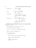
Example 9. Find
()
5f
′
from the following table:
x 124810
f(x) 0152127
Sol. Here the arguments are not equally spaced. So we use Newton’s divide difference
formula.
NUMERICAL DIFFERENTIATION AND INTEGRATION
307
Difference table
x
()
fx
()
fx
∆
()
2
fx
∆
()
3
fx
∆
()

4
fx
∆
10
1
21
1
3
20
45
1
3
1
144
−
4
1
16
−
821
−
1
6
3
10 27
Newton’s divided difference formula is given by:

2
000010012
() ()( )()( )( ) ()( )( )( )

fx fx xx fx xx xx fx xx xx xx=+−∆+−−∆ +−−−
34
001230
()()()()()()
fx xx xx xx xx fx∆ +−−−−∆
(1)
Differentiating (1) w.r.t. x, we get
2 3
0 01 0 12 02 01 0
()()(2 )()[()()()()()()]()
fxfx xxxfx xxxxxxxxxxxx fx
′
=∆ + − − ∆ + − − + − − + − − ∆ +
At x = 5
1
(5) 1 (10 1 2) [(5 2)(5 4) ((5 1)(5 4) (5 1)(5 2)] 0
3
f
′
=+ −− +− −+− −+− −×

1
[(5 2)(5 4)(5 8) (5 1)(5 4)(5 8) (5 1)(5 2)(5 8) (5 1)(5 2)(5 4)]
144
−
+−−−+−−−+−−−+−−−

[]
11 745
17 1

9123612
3 144 3 144
f

′
=+ − =+ +
−− − +


Hence
(5) 3.6458.f
′
=
Ans.
Example 10. Find
(5)f
′′′
from the data given below:
x 2 4 9 13162129
f(x) 57 1345 66340 402052 1118209 4287844 21242820
Sol. Here, the arguments are not equally spaced and therefore we shall apply Newton’s divided
difference formula.
2
000010012
() ()( )()( )( ) ()( )( )( )
fx fx xx fx xx xx fx xx xx xx=+−∆+−−∆ +−−−
34
001230
()()()()()()
fx xx xx xx xx fx∆ +−−−−∆

(1)
308
COMPUTER BASED NUMERICAL AND STATISTICAL TECHNIQUES
x f (x)
()fx∆
2
()
fx∆
()
3
fx∆
()
4
fx∆
5
()
fx∆
6
()
fx∆
257
644
4 1345 1765
12999 556
9 66340 7881 45
83928 1186 1
13 402052 22113 64 0
238719 2274 1
16 1118209 49401 89
633927 4054

21 4287844 114265
2119372
29 21242820
Substituting values in eqn. (1), we get

( ) 57 ( 2)(644) ( 2)( 4)(1765) ( 2)( 4)( 9)(556)fx x x x x x x=+− +− − +− − −

( 2)( 4)( 9)( 13)(45) ( 2)( 4)( 9)( 13)( 16)(1)xxxx xxxx x+−−−− +−−−− −

232
57 644( 2) 1765( 6 8) 556( 15 62 72)
xxxxxx=+ −+ −++ − + −

43 2 54 3 2
45( 28 257 878 936) 44 705 4990
xx x x xx x x+−+−++−+−

14984 14976x+−

232
( ) 644 1765(2 6) 556(3 30 62) 45(4 84 514 878)
fx x x x x x x
′
=+ −+ −++ − + −

43 2
5 176 2115 9980 14984
xx x x+− + − +

232

( ) 3530 556(6 30) 45(12 168 514) 20 528 4230 9980
fx x x x x x x
′′
=+ −+ −++− + −

2
( ) 3336 45(24 168) 60 1056 4230
fx x x x
′′′
=+ −+− +

2
60 24 6
xx=++
Where x = 5;
2
(5) 60(5) 24(5) 6 1626
f
′′′
=++=
. Ans.
Example 11. Find f′(4) from the following data:
x 02 51
()fx
0 8 125 1
Sol. Though this problem can be solved by Newton’s divided difference formula, we are giving
here, as an alternative, Lagrange’s method. Lagrange’s polynomial, in this case, is given by
NUMERICAL DIFFERENTIATION AND INTEGRATION
309
ej

ej
(2)(5)(1) (0)(5)(1)
() (0) (8)
(0 2)(0 5)(0 1) (2 0)(2 5)(2 1)
xxx xxx
fx
−−− −−−
=+
−−− −−−

( 0)( 2)( 1) ( 0)( 2)( 5)
(125) (1)
(5 0)(5 2)(5 1) (1 0)(1 2)(1 5)
xxx xxx
−−− −−−
++
−−− −−−

32 32 32 3
4251
( 6 5) ( 3 2) ( 7 10)
3124
xxx xxx xx xx=− − + + − + + − + =
∴

2
() 3
fx x
′
=

When x = 4, f ′(4) = 3(4)
2
= 48. Ans.
Example 12. Find
(0.6)f
′
and
(0.6)f
′′
from the following table:
x 0.4 0.5 0.6 0.7 0.8
()
fx
1.5836 1.7974 2.0442 2.3275 2.6510
Sol. Here, the derivatives are required at the central point x = 0.6, so we use Stirling’s
formula.
Difference table
uxf(x)
()fx∆
2
()
fx∆
3
()
fx∆
4
()
fx∆
–2 0.4 1.5836
0.2138

–1 0.5 1.7974 0.0330
0.2468 0.0035
0 0.6 (2.0442) (0.0365) (0.0002)
0.2833 0.0037
1 0.7 2.3275 0.0402
0.3235
2 0.8 2.6510
Here we have
0
0
0.6, 0.1, at 0.6, 0
xx
xhu xu
h
−
=== = =
Stirling’s formula is

33
23 42
24
01 1 2
01 2
()
22 6 2 24
yy y y
uuu uu
fx y y u y y
−−−
−−


∆+∆ ∆ +∆
−−

== + + ∆ + + ∆





(1)
Differentiating (1) w.r.t. x, we get
33
23
24
01 1 2
12
13142
( )
26224
yy y y
uuu
fx u y y
h
−−−
−−


∆+∆ ∆ +∆
−−


′
=+∆+ +∆+








310
COMPUTER BASED NUMERICAL AND STATISTICAL TECHNIQUES
ej
ej
Using difference table, we have

23
0111
0.2468, 0.2833, 0.0365, 0.0035,
yy y y
−−−
∆= ∆= ∆= ∆=

34
22
0.0037, 0.0002,
yy
−−
∆= ∆=


0.2468 0.2833 1 0.0035 0.0037 1
(0.6) 0 0
2620.1
f
++


′
=+− +





10[0.26505 0.0006]=−
= f’(0.6) = 2.6445.


Ans.
Again differentiating (1), we get

33
2
2412
12
2
1122
()
224

yy
u
fx y u y
h
−−
−−


∆+∆
−
′′
=∆+ + ∆+







2
11
(0.6) 0.0365 0 0.0002
12
(0.1)
f

′′
=+−×




100[0.0365 0.000016]=−
Hence,
(0.6) 3.6484f
′′
=
Ans.
Example 13. Find
(93)f
′
from the following table:
x 60 75 90 105 120
()
fx
28.2 38.2 43.2 40.9 37.7
Sol. Difference table
u x f (x)
()fx
∆
2
()
fx∆
3
()
fx∆
4
()
fx∆
–2 60 28.2
10 –5

–1 75 38.2
5 –7.3 –2.3
0 90 (43.2) (8.7)
–2.3 –0.9 6.4
1 105 40.9
–3.2
2 120 37.7
Here we have
0
90, 93, 15
xxh===
∴

0
93 90 3 1
0.2
15 15 5
xx
u
h
−
−
== ===
NUMERICAL DIFFERENTIATION AND INTEGRATION
311
Now using Stirling’s formula

33
23 42
24

01 1 2
01 2
()
22 6 2 24
yy y y
uuu uu
fx y y u y y
−−−
−−

∆+∆ ∆ +∆
−−

== + + ∆ + + ∆ +





(1)
Differentiating (1) w.r.t. x, we get
()
33
23
24
01 1 2
12
13142

26224

yy y y
uuu
fx u y y
h
−−−
−−


∆+∆ ∆ +∆
−−

′
=+∆+ +∆+








Putting the values of x = 93, u = 0.2, h = 15 and

23 34
01 1 1 2 2
5, 2.3, 7.3 2.3, 6.4, 8.7
yy y y y y
−−−−−
∆=∆ =− ∆ =− ∆ =− ∆ = ∆ =
We get,

23
1 5 2.3 3(0.2) 1 2.3 6.4 4(0.2) 2(0.2)
(93) 0.2( 7.3) (8.7)
15 2 6 2 24
f

− −−+ −

′
=+−+ +




1 2.7 3.608 3.2016
1.46
15 2 6 2 24

=−−−

×

1 0.6013
1.35 1.46 0.1334
15 2

=−−−


[]

1
1.35 1.46 0.30065 0.1334
15
=−−−
(93) 0.03627f
′
=−
. Ans.
Example 14. Find x for which y is maximum and find this value of y
x 1.2 1.3 1.4 1.5 1.6
y 0.9320 0.9636 0.9855 0.9975 0.9996
Sol. The Difference table is as follows:
xu∆∆
2
∆
3
∆
4
1.2 0.9320
0.0316
1.3 0.9636 –0.0097
0.0219 –0.0002
1.4 0.9855 –0.0099 0.0002
0.0120 0
1.5 0.9975 –0.0099
0.0021
1.6 0.9996
312
COMPUTER BASED NUMERICAL AND STATISTICAL TECHNIQUES
Let

0
y
=0.9320 and a = 1.2
By Newton’s forward difference formula

2
00 0
(1)

2
uu
yy uy y
−
=+∆+ ∆ +

(1)
0.9320 0.0316 (–0.0097)
2
uu
u
−
=+ +
(Neglecting higher differences)

21
0.0316 (–0.0097)
2
dy
u
du

−

=+


At a maximum,

0
dy
du
=
⇒
1
0.0316 (0.0097) 3.76
2
uu

=− ⇒=


∴

0
1.2 (0.1)(3.76) 1.576
xx hu=+= + =
To find
max ,
y
we use backward difference formula,
x = x

n
+ hu
⇒

1.576 1.6 (0.1) 0.24uu=+ ⇒=−

23
(1) (1)(2)
(1.576)
2! 3!
nn n n
uu uu u
yyuy y y
+++
=+∇+ ∇ + ∇

(–0.24)(1– 0.24)
0.9996 (0.24 0.0021) (–0.0099)
2
=−×+

0.9999988 0.9999==
nearly
∴
Maximum y = 0.9999. (Approximately)


Ans.
Example 15. From the following table, for what value of x, y is minimum. Also find this value of y.
x 34 56 7 8

y 0.205 0.240 0.259 0.260 0.250 0.224
Sol. Difference table
xy ∆∆
2
∆
3
3 0.205
0.035
4 0.240 –0.016
0.019 0.000
5 0.259 –0.016
0.003 0.001
6 0.262 –0.015
–0.012 0.001
7 0.250 –0.014
–0.026
8 0.224
NUMERICAL DIFFERENTIATION AND INTEGRATION
313
Now taking x
0
= 3, we have
2
00 0
0.205, 0.035, 0.016
yy y=∆= ∆=−
and
3
0
0

y∆=
.
Therefore, Newton’s forward interpolation formula gives

(1)
0.205 (0.035) ( 0.016)
2
uu
yu
−
=+ − −
(1)
Differentiating (1), w.r.t. u, we get

21
0.035 (–0.016)
2
dy
u
du
−
=+
For y to be minimum put
0
dy
du
=
⇒
0.035 – 0.008(2 1) 0u−=
⇒

2.6875u =
Therefore,
0
xx uh=+

3 2.6875 1 5.6875=+ ×=
Hence, y is minimum when x = 5.6875.
Putting u = 2.6875 in (1), we get the minimum value of y given by

1
0.205 2.6875 0.035 (2.6875 1.6875)(–0.016)
2
=+ ×+ ×
= 0.2628. Ans.
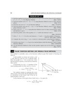
PROBLEM SET 6.1
1. Find
(6)
′
f
from the following table:
()
0134 5 7 9
150 108 0 54 100 144 84
x
fx −−−−
[Ans. –23]
2. Use the following data to find f ′(3):
()
3 5 11 27 34
13 28 899 17315 35606

x
fx −
[Ans. 1.8828]
3. Use the following data to find f ′(5):
()
24 9 10
4 56 711 980
x
fx
[Ans. 2097.69]
4. From the table, find
dy
dx
at x = 1, x = 3 and x = 6:
()
0123456
6.9897 7.4036 7.7815 8.1291 8.4510 8.7506 9.0309
x
fx
[Ans. 0.3952, 0.3341, 0.2719]
314
COMPUTER BASED NUMERICAL AND STATISTICAL TECHNIQUES
5. Find f ′(5) and f ′′(5) from the following data:
()
24 9 13
57 1345 66340 402052
x
fx
6. Using Newton’s Divided Difference Formula, find f ′(10) from the following data:
()

3 5 11 27 34
13 23 99 17315 35606
x
fx −
[Ans. 232.869]
7. From the table below, for what value of x, y is minimum? Also find this value of y.
345678
4 0.205 0.240 0.259 0.262 0.250 0.224
x
[Ans. 5.6875, 0.2628]
8. A slider in a machine moves along a fixed straight rod. Its distance x (in cm.) along the rod is
given at various times t (in secs.)
0 0.1 0.2 0.3 0.4 0.5 0.6
30.28 31.43 32.98 33.54 33.97 33.48 32.13
t
x
Evaluate
dx
dt
at t = 0.1 and at t = 0.5 [Ans. 32.44166 cm/sec.; −24.05833 cm/sec.]
9. A rod is rotating in a plane. The following table gives the angle
θ
(radians) through which
the rod has turned for various values of the time t (seconds).
0 0.2 0.4 0.6 0.8 1.0 1.2
0 0.12 0.49 1.12 2.02 3.20 4.67
t
θ
Calculate the angular velocity and acceleration of the rod when t = 0.6 sec.
[Ans. (i) 3.82 radians/sec. (ii) 6.75 radians/sec

2
]
10. The table given below reveals the velocity ‘v’ of a body during the time ‘t’ specified. Find its
acceleration at t = 1.1.
1.0 1.1 1.2 1.3 1.4
43.1 47.7 52.1 56.4 60.8
t
v
[Ans. 44.92]
NUMERICAL DIFFERENTIATION AND INTEGRATION
315
6.3 NUMERICAL INTEGRATION
Like numerical differentiation, we need to seek the help of numerical integration techniques in the
following situations:
1. Functions do not possess closed from solutions. Example:
2
–
0
()
x
t
fx C e dt
=
∫
.
2. Closed form solutions exist but these solutions are complex and difficult to use for
calculations.
3. Data for variables are available in the form of a table, but no mathematical relationship
between them is known as is often the case with experimental data.
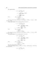
6.4 GENERAL QUADRATURE FORMULA

Let
()yfx=
be a function, where y takes the values y
0
, y
1
, y
2
, y
n
for x = x
0
, x
1
, x
2
, x
n
. We
want to find the vaule of
()
b
a
Ifxdx
=
∫
.
Let the interval of integration (a, b) be divided into n equal subintervals of width
ba
h

n
−

=


so
that
01020 0
, , 2 , ,
n
xaxxhxx hT xxnhb
==+=+ =+=
.
∴

0
0
() ()
nh
x
b
ax
I f xdx fxdx
+
==
∫∫
(1)
Newton’s forward interpolation formula is given by


23
00 0 0
(1) (–1)(2)
( )
2! 3!
uu uu u
yfx y uy y y
−−
==+∆+ ∆+ ∆+
Where
0
xx
u
h
−
=
∴

1
du dx dx hdu
h
=⇒=
∴
Equation (1) becomes,

23
00 0 0
0
(1) (1)(2)


2! 3!
n
uu uu u
Ihy uy y y du
−−−

=+∆+ ∆+ ∆+


∫

2
23
00 0 0
(2 3) ( 2)
up to( 1) terms
212 24
nnn nn
nh y y y y n

−−
= +∆+ ∆+ ∆+ + +


∴

0
2
23
00 0 0

(2 3) ( 2)
( ) up to ( 1) terms
212 24
n
x
x
nnn nn
f x dx nh y y y y n

−−
= +∆+ ∆+ ∆+ + +


∫
(2)
This is called general quadrature formula.