DISCRETE-SIGNAL ANALYSIS AND DESIGN- P7 doc
Bạn đang xem bản rút gọn của tài liệu. Xem và tải ngay bản đầy đủ của tài liệu tại đây (144.73 KB, 5 trang )
16 DISCRETE-SIGNAL ANALYSIS AND DESIGN
part and an imaginary part, the real parts add coherently and the imaginary
parts add coherently, and the power is complex (real watts and imaginary
vars). There is much more about this later.
If K
x
=1.2 in Eq. (1-1), then 1.2 cycles would be visible, the spectrum
would contain many frequencies, and the Þnal phase would change to
(0.2 · 2π) radians. The value of the phase angle in degrees for each
complex X (k)is
φ(k) = arctan
Im
X(k)
Re
X(k)
·
180
π
degrees (1-3)
For an example of this type of sequence, look ahead to Fig. 1-6. A later
section of this chapter gives more details on complex frequency-domain
sequences.
At this point, notice that the complex term exp(j ωt) is calculated by
Mathcad using its powerful and efÞcient algorithms, eliminating the need
for an elaborate complex Taylor series expansion by the user at each value
of (n)or(ω). This is good common sense and does not derail us from
our discrete time/frequency objectives.
At each (k) stop, the sum is performed at 0 to N −1 values of time (n),
for a total of N values. It may be possible to evaluate accurately enough
the sum at each (k) value with a smaller number of time steps, say N /2
or N /4. For simplicity and best accuracy, N will be used for both (k)
and (n). Using Mathcad to Þnd the spectrum without assigning discrete
(k) values from 0 to N −1, a very large number of frequency values are
evaluated and a continuous graph plot is created. We will do this from
time to time, and the summation () becomes more like an integral
,
but this is not always a good idea, for reasons to be seen later.
Note also that in Eq. (1-2) the factor 1/N ahead of the sum and the
minus sign in the exponent are used but are not used in Eq. (1-8) (look
ahead). This notation is common in engineering applications as described
by [Ronald Bracewell, 1986] and is also an option in Mathcad (functions
FFT and IFFT). See also [Oppenheim and Willsky et al., 1983, p. 321].
This agrees with the practical engineering emphasis of this book. It also
agrees with our assumption that each record, 0 to N −1, is one replication
of an inÞnite steady-state signal. These two equations, used together and
consistently, produce correct results.
FIRST PRINCIPLES 17
Each (k ) is a harmonic number for the frequency sequence X (k). To
repeat a few previous statements for emphasis, k =1 is the fundamen-
tal frequency, k =2 is second harmonic, etc. A two-sided (positive and
negative) phasor spectrum is produced by this equation (we will learn to
appreciate the two-sided spectrum concept). N , an integral power of 2,
is chosen large enough to provide adequate resolution of the spectrum
(sufÞcient harmonics of k =1). The dc component is at k =0[wherethe
exp(0) term =1.0] and
X(0) =
1
N
N−1
n=0
x(n) =x(n) volts (1-4)
which is the time average over the entire sequence, 1.0, in Fig. 1-2.
Equation (1-2) can be used directly to get the spectrum, but as a matter
of considerable interest later it can be separated into two regions having
an equal number of data points, from 0 to N /2 −1 and from N /2 to N −1
as shown in Eq. (1-5). If N =8, then k (positive frequencies) =1, 2, 3 and
k (negative frequencies) =7, 6, 5. Point N is the beginning of the next
periodic continuation. Dc is at k =0, and N /2 is not used, for reasons to
be explained later in this chapter.
Consider the following manipulations of Eq. (1-2):
X(k) =
1
N
⎡
⎣
N/2−1
n=0
x(n)e
−jk2π
(
n
N
)
+
N−1
n=N/2
x(n)e
−jk2π
(
n
N
)
⎤
⎦
(1-5)
The last exponential can be modiÞed as follows without changing its
value:
e
−jk2π
n
N
= e
j(2πn)
360
◦
e
−jk2π
n
N
= e
j2πn
1−
k
N
= e
j2π
(
N−k
)
n
N
(1-6)
and Eq. (1-2) becomes
X(k) =
1
N
⎡
⎣
N/2−1
n=0
x(n)e
−jk2π
n
N
+
N−1
n=N/2
x(n)e
j2π(N−k)
n
N
⎤
⎦
(1-7)
18 DISCRETE-SIGNAL ANALYSIS AND DESIGN
The second exponential is the phase conjugate (e
−jθ
→e
+jθ
)oftheÞrst
and is positioned as shown in Fig. 1-2b for k =N /2 to N −1. At k =0
we see the dc. The two imaginary components −j 0.5 and +j 0.5, are at
k =1andk =63 (same as k =−1), typical for a sine wave of length
64. We use this method quite often to convert two-sided sequences into
one-sided (positive-time or positive-frequency) sequences (see Chapter 2
for more details).
INVERSE DISCRETE FOURIER TRANSFORM
The inverse transformation (IDFT) in Eq. (1-8) [Oppenheim et al., 1983,
p. 321] takes the two-sided spectrum X (k ) in Fig. 1-2b and exactly recre-
ates the original two-sided time sequence x(n) shown in Fig. 1-2c:
x(n) =
N−1
k=0
X(k)e
jk2π
(
n
N
)
(1-8)
At each value of (n) the spectrum values X (k ) are summed from k =0to
k =N −1. In Eq. (1-8) the phase increments are in the counter-clockwise
(positive) direction. This reverses the negative phase increments that were
introduced into the DFT [Eq. (1-2)]. This step helps to return each complex
X (k ) in the frequency domain to a real x(n) in the time domain. See further
discussion later in the chapter.
It is interesting to focus our attention on Eqs. (1-2) and (1-8) and to
observe that in both cases we are simultaneously in the time and frequency
domains. We must have data from both domains to travel back and forth.
This conÞrms that we are learning to be comfortable in both domains at
once, which is exactly what we need to do.
So far, Eqs. (1-2) and (1-8) have been used directly, without any need
for a faster method, the FFT (the Fast Fourier Transform), described later.
Modern personal computers are usually fast enough for simple problems
using just these two equations. Also, Eqs. (1-2) and (1-8) are quite accurate
and very easy to use in computerized analysis (however, Mathcad also
has very excellent tools for numerical and symbolic integration that we
will use frequently). We do not have to worry about those two discrete
FIRST PRINCIPLES 19
equations in our applications because they have been thoroughly tested.
It is a good idea to use Eqs. (1-2) and (1-8) together as a pair. To narrow
the time or frequency resolution, multiply the value of N by 2
M
(m =1,
2, 3, ), as shown in the next section.
FREQUENCY AND TIME SCALING
Suppose a signal spectrum extends from 0 Hz to 30 MHz (Fig. 1-3) and we
want to display it as a 32-point (=2
5
) two-sided spectrum. The positive
side of the spectrum has 15 X (k ) values from 1 to N /2 −1 (not count-
ing 0 and N /2), and the negative side of the spectrum also has 15 X (k )
values from N /2 +1toN −1 (not counting N /2 and N ). The frequency
range 0 to 30 MHz consists of a fundamental frequency k
1
and 2
4
−1 =15
harmonics of k
1
. The fundamental frequency k1 is determined by
k
1
·15 = 3·10
7
∴ k
1
=
3·10
7
15
= 2 MHz (1-9)
and this is the best resolution of frequency that can be achieved with
15 points (positive or negative frequencies) of a 30-MHz signal using
a 32-point two-sided spectrum. If we use 2048 data points, we can get
29.31551-kHz resolution using Eq. (1-9).
+/− 30 MHz
0
0
2.0 MHz resolution
K=
+1
K = −1
−2 MHz
Figure 1-3 A 30-MHz two-sided spectrum with 32 frequency samples,
including 0.
20 DISCRETE-SIGNAL ANALYSIS AND DESIGN
An excellent way to improve this example is to frequency-convert the
signal band to a much lower frequency, for example 3 MHz, using a very
stable local oscillator, which would give us a 2931.55- Hz resolution for
this example. Increasing the samples to 2
14
at 3 MHz provides a resolution
of 366.26 Hz, and so forth for higher sample numbers. This is basically
what spectrum analyzers do.
The good news for this problem is that a hardware frequency translator
may not be necessary. If the signal is narrowband, such as speech or
low-speed data or some other bandlimited process, the original 30-MHz
problem might be restated at 3 MHz, or maybe even at 0.3 MHz, with the
same signal bandwidth and with no loss of correct results, but with greatly
improved resolution. With programs for personal computer analysis, very
large numbers of samples are not desirable; therefore, we do not try to
push the limits too much. The waveform analysis routines usually tell
us what we want to know, using more reasonable numbers of samples.
Designing the frequency and time scales is very helpful.
Consider a time scaling example, a sequence (record length) that is
10 μsec long from start of one sequence to the start of the next sequence,
as shown in Fig. 1-4. For N =4 there are 4 time values (0, 1, 2, 3) and
4 time intervals (1, 2, 3, 4) to the beginning of the next sequence, which
is 10
−5
/4 =2.5 μsec per interval. In the Þrst half there are 2 intervals
for a total of 5.0 μsec. For the second half there are also 2 intervals, for
a total of 5.0 μsec. Each interval is a “band” of possibly smaller time
increments. The total time is 10.0 μsec.
01 2 3
1
2
3
4
0 2.5
+5.0
− 5.0 −2.5
0
N = 4
msec
10 msec
Figure 1-4 A 10-μsec time sequence with positive and negative time
values.