420 G. Peter Zhang
The popularity of neural networks is due to their powerful modeling capability
for pattern recognition. Several important characteristics of neural networks make
them suitable and valuable for data mining. First, as opposed to the traditional model-
based methods, neural networks do not require several unrealistic a priori assump-
tions about the underlying data generating process and specific model structures.
Rather, the modeling process is highly adaptive and the model is largely determined
by the characteristics or patterns the network learned from data in the learning pro-
cess. This data-driven approach is ideal for real world data mining problems where
data are plentiful but the meaningful patterns or underlying data structure are yet to
be discovered and impossible to be pre-specified.
Second, the mathematical property of the neural network in accurately approxi-
mating or representing various complex relationships has been well established and
supported by theoretic work (Chen and Chen, 1995; Cybenko, 1989; Hornik, Stinch-
combe, and White 1989). This universal approximation capability is powerful be-
cause it suggests that neural networks are more general and flexible in modeling the
underlying data generating process than traditional fixed-form modeling approaches.
As many data mining tasks such as pattern recognition, classification, and forecast-
ing can be treated as function mapping or approximation problems, accurate identi-
fication of the underlying function is undoubtedly critical for uncovering the hidden
relationships in the data.
Third, neural networks are nonlinear models. As real world data or relationships
are inherently nonlinear, traditional linear tools may suffer from significant biases
in data mining. Neural networks with their nonlinear and nonparametric nature are
more cable for modeling complex data mining problems.
Finally, neural networks are able to solve problems that have imprecise patterns
or data containing incomplete and noisy information with a large number of vari-
ables. This fault tolerance feature is appealing to data mining problems because real
data are usually dirty and do not follow clear probability structures that typically
required by statistical models.
This chapter aims to provide readers an overview of neural networks used for

data mining tasks. First, we provide a short review of major historical developments
in neural networks. Then several important neural network models are introduced
and their applications to data mining problems are discussed.
21.2 A Brief History
Historically, the field of neural networks is benefited by many researchers in di-
verse areas such as biology, cognitive science, computer science, mathematics, neu-
roscience, physics, and psychology. The advancement of the filed, however, is not
evolved steadily, but rather through periods of dramatic progress and enthusiasm and
periods of skepticism and little progress.
The work of McCulloch and Pitts (1943) is the basis of modern view of neural
networks and is often treated as the origin of neural network field. Their research
is the first attempt to use mathematical model to describe how a neuron works. The
21 Neural Networks For Data Mining 421
main feature of their neuron model is that a weighted sum of input signals is com-
pared to a threshold to determine the neuron output. They showed that simple neural
networks can compute any arithmetic or logical function.
In 1949, Hebb (1949) published his book “The Organization of Behavior.” The
main premise of this book is that behavior can be explained by the action of neurons.
He proposed one of the first learning laws that postulated a mechanism for learning
in biological neurons.
In the 1950s, Rosenblatt and other researchers developed a class of neural net-
works called the perceptrons which are models of a biological neuron. The percep-
tron and its associated learning rule (Rosenblatt, 1958) had generated a great deal
of interest in neural network research. At about the same time, Widrow and Hoff
(1960) developed a new learning algorithm and applied it to their ADALINE (Adap-
tive Linear Neuron) networks which is very similar to perceptrons but with linear
transfer function, instead of hard-limiting function typically used in perceptrons.
The Widrow-Hoff learning rule is the basis of today’s popular neural network learn-
ing methods. Although both perceptrons and ADALINE networks have achieved
only limited success in pattern classification because they can only solve linearly-

separable problems, they are still treated as important work in neural networks and
an understanding of them provides the basis for understanding more complex net-
works.
The neural network research was hit by the book “Perceptrons” by Minsky and
Papert (1969) who pointed out the limitation of the perceptrons and other related
networks in solving a large class of nonlinearly separable problems. In addition, al-
though Minsky and Papert proposed multilayer networks with hidden units to over-
come the limitation, they were not able to find a way to train the network and stated
that the problem of training may be unsolvable. This work causes much pessimism in
neural network research and many researchers have left the filed. This is the reason
that during the 1970s, the filed has been essentially dormant with very little research
activity.
The renewed interest in neural network started in the 1980s when Hopfield (1982)
used statistical mechanics to explain the operations of a certain class of recurrent
network and demonstrated that neural networks could be trained as an associative
memory. Hopfield networks have been used successfully in solving the Traveling
Salesman Problem which is a constrained optimization problem (Hopfield and Tank,
1985). At about the same time, Kohonen (1982) developed a neural network based on
self-organization whose key idea is to represent sensory signals as two-dimensional
images or maps. Kohonen’s networks, often called Kohonen’s feature maps or self-
organizing maps, organized neighborhoods of neurons such that similar inputs into
the model are topologically close. Because of the usefulness of these two types of
networks in solving real problems, more research was devoted to neural networks.
The most important development in the field was doubtlessly the invention of
efficient training algorithms—called backpropagation—for multilayer perceptrons
which have long been suspected to be capable of overcoming the linear separability
limitation of the simple perceptron but have not been used due to lack of good train-
ing algorithms. The backpropagation algorithm, originated from Widrow and Hoff’s
422 G. Peter Zhang
learning rule, formalized by Werbos (1974), developed by Parker (1985), Rumelhart

Hinton, and Williams (Rumelhart Hinton & Williams, 1986) and others, and popu-
larized by Rumelhart, et al. (1986), is a systematic method for training multilayer
neural networks. As a result of this algorithm, multilayer perceptrons are able to
solve many important practical problems, which is the major reason that reinvigo-
rated the filed of neural networks. It is by far the most popular learning paradigm in
neural networks applications.
Since then and especially in the 1990s, there have been significant research activ-
ities devoted to neural networks. In the last 15 years or so, tens of thousands of papers
have been published and numerous successful applications have been reported. It will
not be surprising to see even greater advancement and success of neural networks in
various data mining applications in the future.
21.3 Neural Network Models
As can be seen from the short historical review of development of the neural network
field, many types of neural networks have been proposed. In fact, several dozens of
different neural network models are regularly used for a variety of problems. In this
section, we focus on three better known and most commonly used neural network
models for data mining purposes: the multilayer feedforward network, the Hopfield
network, and the Kohonen’s map. It is important to point out that there are numerous
variants of each of these networks and the discussions below are limited to the basic
model formats.
21.3.1 Feedforward Neural Networks
The multilayer feedforward neural networks, also called multi-layer perceptrons
(MLP), are the most widely studied and used neural network model in practice. Ac-
cording to Wong, Bodnovich, and Selvi (1997), about 95% of business applications
of neural networks reported in the literature use this type of neural model. Feedfor-
ward neural networks are ideally suitable for modeling relationships between a set
of predictor or input variables and one or more response or output variables. In other
words, they are appropriate for any functional mapping problem where we want to
know how a number of input variables affect the output variable(s). Since most pre-
diction and classification tasks can be treated as function mapping problems, the

MLP networks are very appealing to data mining. For this reason, we will focus
more on feedforward networks and many issues discussed here can be extended to
other types of neural networks.
Model Structure
An MLP is a network consisted of a number of highly interconnected simple com-
puting units called neurons, nodes, or cells, which are organized in layers. Each neu-
ron performs simple task of information processing by converting received inputs
21 Neural Networks For Data Mining 423
into processed outputs. Through the linking arcs among these neurons, knowledge
can be generated and stored as arc weights regarding the strength of the relation-
ship between different nodes. Although each neuron implements its function slowly
and imperfectly, collectively a neural network is able to perform a variety of tasks
efficiently and achieve remarkable results.
Figure 21.1 shows the architecture of a three-layer feedforward neural network
that consists of neurons (circles) organized in three layers: input layer, hidden layer,
and output layer. The neurons in the input nodes correspond to the independent or
predictor variables that are believed to be useful for predicting the dependent vari-
ables which correspond to the output neurons. Neurons in the input layer are passive;
they do not process information but are simply used to receive the data patterns and
then pass them into the neurons into the next layer. Neurons in the hidden layer are
connected to both input and output neurons and are key to learning the pattern in
the data and mapping the relationship from input variables to the output variable.
Although it is possible to have more than one hidden layer in a multilayer networks,
most applications use only one layer. With nonlinear transfer functions, hidden neu-
rons can process complex information received from input neurons and then send
processed information to output layer for further processing to generate outputs. In
feedforward neural networks, the information flow is one directional from the input
to hidden then to output layer and there is no feedback from the output.
Input Layer
Hidden Layer

Output Layer
Weights (
w
1
)
Weights (w
2
)
Outputs (y)
Inputs (
x)

Fig. 21.1. Multi-layer feedforward neural network
Thus, a feedforward multilayer neural network is characterized by its architecture
determined by the number of layers, the number of nodes in each layer, the transfer
function used in each layer, as well as how the nodes in each layer connected to nodes
in adjacent layers. Although partial connection between nodes in adjacent layers and
direct connection from input layer to output layer are possible, the most commonly
used neural network is so called fully connected one in that each node at one layer is
fully connected only to all nodes in the adjacent layers.
To understand how the network in Figure 21.1 works, we need first understand
the way neurons in the hidden and output layers process information. Figure 21.2
provides the mechanism that shows how a neuron processes information from several
inputs and then converts it into an output. Each neuron processes information in two
424 G. Peter Zhang
steps. In the first step, the inputs (x
i
) are combined together to form a weighted sum
of inputs and the weights (w
i

) of connecting links. The 2
nd
step then performs a
transformation that converts the sum to an output via a transfer function. In other
words, the neuron in Figure 21.2 performs the following operations:
Out
n
= f

∑
i
w
i
x
i

, (21.1)
where Out
n
is the output from this particular neuron and f is the transfer function. In
general, the transfer function is a bounded nondecreasing function. Although there
are many possible choices for transfer functions, only a few of them are commonly
used in practice. These include
1. the sigmoid (logistic) function, f (x)=(1 + exp(−x))
−1
,
2. the hyperbolic tangent function, f (x)=
exp(x)−exp(−x)
exp(x)+exp(−x)
,

3. the sine and cosine function, f (x)=sin(x), f (x)=cos(x), and
4. the linear or identity function, f (x)=x.
Among them, the logistic function is the most popular choice especially for the
hidden layer nodes due to the fact that it is simple, has a number of good char-
acteristics (bounded, nonlinear, and monotonically increasing), and bears a better
resemblance to real neurons (Hinton, 1992).
Sum
Trans-
form
w 1
x
1

x
2

x
3

x
d

w 2
w 3
w
d
I
n
p
u

t
Output

Fig. 21.2. Information processing in a single neuron
In Figure 21.1, let x =(x
1
,x
2
, ,x
d
) be a vector of d predictor or attribute vari-
ables, y =(y
1
,y
2
, ,y
M
)be the M-dimensional output vector from the network, and
w
1
and w
2
be the matrices of linking arc weights from input to hidden layer and from
hidden to output layer, respectively. Then a three-layer neural network can be written
as a nonlinear model of the form
y = f
2
(w
2
f

1
(w
1
x)), (21.2)
where f
1
and f
2
are the transfer functions for the hidden nodes and output nodes
respectively. Many networks also contain node biases which are constants added to
21 Neural Networks For Data Mining 425
the hidden and/or output nodes to enhance the flexibility of neural network modeling.
Bias terms act like the intercept term in linear regression.
In classification problems where desired outputs are binary or categorical, lo-
gistic function is often used in the output layer to limit the range of the network
outputs. On the other hand, for prediction or forecasting purposes, since output vari-
ables are in general continuous, linear transfer function is a better choice for out-
put nodes. Equation (63.2) can have many different specifications depending on the
problem type, the transfer function, and numbers of input, hidden, and output nodes
employed. For example, the neural network structure for a general univariate fore-
casting problem with logistic function for hidden nodes and identity function for the
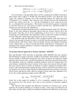
output node can be explicitly expressed as
y
t
= w
10
+
q
∑
j=1

w
1 j
f (
p
∑
i=1
w
ij
x
it
+ w
0 j
) (21.3)
where y
t
is the observation of forecast variable and {x
it
, i = 1, 2, , p} are p pre-
dictor variables at time t, p is also the number of input nodes, q is the number of
hidden nodes, {w
1 j
, j = 0, 1, , n} are weights from the hidden to output nodes and
{w
ij
,i = 0,1, , p; j = 1,2, ,q} are weights from the input to hidden nodes;
α
0
and
β
0 j

are bias terms, and f is the logistic function defined above.
Network Training
The arc weights are the parameters in a neural network model. Like in a statistical
model, these parameters need to be estimated before the network can be adopted for
further use. Neural network training refers to the process in which these weights are
determined, and hence is the way the network learns. Network training for classifi-
cation and prediction problems is performed via supervised learning in which known
outputs and their associated inputs are both presented to the network.
The basic process to train a neural network is as follows. First, the network is
fed with training examples, which consist of a set of input patterns and their desired
outputs. Second, for each training pattern, the input values are weighted and summed
at each hidden layer node and the weighted sum is then transmitted by an appropriate
transfer function into the hidden node’s output value, which becomes the input to the
output layer nodes. Then, the network output values are calculated and compared
to the desired or target values to determine how closely the actual network outputs
match the desired outputs. Finally, the weights of the connection are changed so that
the network can produce a better approximation to the desired output. This process
typically repeats many times until differences between network output values and
the known target values for all training patterns are as small as possible.
To facilitate training, some overall error measure such as the mean squared errors
(MSE) or sum of squared errors (SSE) is often used to serve as an objective function
or performance metric. For example, MSE can be defined as
426 G. Peter Zhang
MSE =
1
M
1
N
M
∑

m=1
N
∑
j=1
(d
mj
−y
mj
)
2
, (21.4)
where d
mj
and y
mj
represent the desired (target) value and network output at the mth
node for the jth training pattern respectively, M is the number of output nodes, and
N is the number of training patterns. The goal of training is to find the set of weights
that minimize the objective function. Thus, network training is actually an uncon-
strained nonlinear optimization problem. Numerical methods are usually needed to
solve nonlinear optimization problems.
The most important and popular training method is the backpropagation algo-
rithm which is essentially a gradient steepest descent method. The idea of steepest
descent method is to find the best direction in the multi-dimension error space to
move or change the weights so that the objective function is reduced most. This re-
quires partial derivative of the objective function with respect to each weight to be
calculated because the partial derivative represents the rate of change of the objective
function. The weight updating therefore follows the following rule
w
new

ij
= w
old
ij
+
Δ
w
ij
Δ
w
ij
= −
η
∂
E
∂
w
ij
(21.5)
where
Δ
w
ij
is the gradient of objective function E with respect to weight w
ij
, and
η
is called the learning rate which controls the size of the gradient descent step. The
algorithm requires an iterative process and there are two versions of weight updating
schemes: batch mode and on-line mode. In the batch mode, weights are updated after

all training patterns are evaluated, while in the on-line learning mode, the weights are
updated after each pattern presentation. The basic steps with the batch mode training
can be summarized as
initialize the weights to small random values from, say, a uniform distribution
choose a pattern and forward propagate it to obtain network outputs
calculate the pattern error and back-propagate it to obtain partial derivative of this
error with respect to all weights
add up all the single-pattern terms to get the total derivative
update the weights with equation (63.6)
repeat steps 2-5 for next pattern until all patterns are passed through.
Note that each one pass of all patterns is called an epoch. In general, each weight
update reduces the total error by only a small amount so many epochs are often
needed to minimize the error. For information on further detail of the backpropaga-
tion algorithm, readers are referred to Rumelhart et al. (1986) and Bishop (1995).
It is important to note that there is no algorithm currently available which can
guarantee global optimal solution for general nonlinear optimization problems such
as those in neural network training. In fact, all algorithms in nonlinear optimization
inevitably suffer from the local optima problems and the most we can do is to use
the available optimization method which can give the ”best” local optima if the true
global solution is not available. It is also important to point out that the steepest
descent method used in the basic backpropagation suffers the problems of slow con-
vergence, inefficiency, and lack of robustness. Furthermore, it can be very sensitive
21 Neural Networks For Data Mining 427
to the choice of the learning rate. Smaller learning rates tend to slow the learning pro-
cess while larger learning rates may cause network oscillation in the weight space.
Common modifications to the basic backpropagation include adding in the weight
updating formula (63.1) an additional momentum parameter proportional to the last
weight change the to control the oscillation in weight changes and (63.2) a weight
decay term that penalizes the overly complex network with large weights.
In light of the weakness of the standard backpropagation algorithm, the existence

of many different optimization methods (Fletcher, 1987) provides various alterna-
tive choices for the neural network training. Among them, the second-order methods
such as BFGS and Levenberg-Marquardt methods are more efficient nonlinear opti-
mization methods and are used in most optimization packages. Their faster conver-
gence, robustness, and the ability to find good local minima make them attractive in
neural network training. For example, De Groot and Wurtz (1991) have tested sev-
eral well-known optimization algorithms such as quasi-Newton, BFGS, Levenberg-
Marquardt, and conjugate gradient methods and achieved significant improvements
in training time and accuracy.
Modeling Issues
Developing a neural network model for a data mining application is not a trivial
task. Although many good software packages exist to ease users’ effort in building a
neural network model, it is still critical for data miners to understand many important
issues around the model building process. It is important to point out that building a
successful neural network is a combination of art and science and software alone is
not sufficient to solve all problems in the process. It is a pitfall to blindly throw data
into a software package and then hope it will automatically identify the pattern or
give a satisfactory solution. Other pitfalls readers need to be cautious can be found
in Zhang (2007).
An important point in building an effective neural network model is the under-
standing of the issue of learning and generalization inherent in all neural network
applications. This issue of learning and generalization can be understood with the
concepts of model bias and variance (Geman, Bienenstock & Doursat, 1992). Bias
and variance are important statistical properties associated with any empirical model.
Model bias measures the systematic error of a model in learning the underlying rela-
tions among variables or observations. Model variance, on the other hand, relates to
the stability of a model built on different data samples and therefore offers insights
on generalizability of the model. A pre-specified or parametric model, which is less
dependent on the data, may misrepresent the true functional relationship and hence
cause a large bias. On the other hand, a flexible, data-driven model may be too de-

pendent on the specific data set and hence have a large variance. Bias and variance
are two important terms that impact a model’s usefulness. Although it is desirable
to have both low bias and low variance, we may not be able to reduce both terms
at the same time for a given data set because these goals are conflicting. A model
that is less dependent on the data tends to have low variance but high bias if the pre-
specified model is incorrect. On the other hand, a model that fits the data well tends
428 G. Peter Zhang
to have low bias but high variance when applied to new data sets. Hence a good pre-
dictive model should have an “appropriate” balance between model bias and model
variance.
As a data-driven approach to data mining, neural networks often tend to fit the
training data well and thus have low bias. But the potential price to pay is the overfit-
ting effect that causes high variance. Therefore, attentions should be paid to address
issues of overfitting and the balance of bias and variance in neural network model
building.
The major decisions in building a neural network model include data preparation,
input variable selection, choice of network type and architecture, transfer function,
and training algorithm, as well as model validation, evaluation, and selection proce-
dures. Some of these can be solved during the model building process while others
must be considered before actual modeling starts.
Neural networks are data-driven techniques. Therefore, data preparation is a crit-
ical step in building a successful neural network model. Without an adequate and
representative data set, it is impossible to develop a useful data mining model.
There are several practical issues around the data requirement for a neural net-
work model. The first is the data quality. As data sets used for typical data mining
tasks are massive and may be collected from multiple sources, they may suffer many
quality problems such as noises, errors, heterogeneity, and missing observations. Re-
sults reported in Klein and Rossin (1999) suggest that data error rate and its magni-
tude can have substantial impact on neural network performance. Klein and Rossion
believe that an understanding of errors in a dataset should be an important consid-

eration to neural network users and efforts to lower error rates are well deserved.
Appropriate treatment of these problems to clean the data is critical for successful
application of any data mining technique including neural networks (Dasu and John-
son, 2003).
Another one is the size of the sample used to build a neural network. While there
is no specific rule that can be followed for all situations, the advantage of having large
samples should be clear because not only do neural networks have typically a large
number of parameters to estimate, but also it is often necessary to split data into sev-
eral portions for overfitting prevention, model selection, evaluation, and comparison.
A larger sample provides better chance for neural networks to adequately approxi-
mate the underlying data structure.
The third issue is the data splitting. Typically for neural network applications, all
available data are divided into an in-sample and an out-of-sample. The in-sample data
are used for model fitting and selection, while the out-of-sample is used to evaluate
the predictive ability of the model. The in-sample data often are further split into
a training sample and a validation sample. The training sample is used for model
parameter estimation while the validation sample is used to monitor the performance
of neural networks and help stop training and select the final model. For a neural
network to be useful, it is critical to test the model with an independent out-of-sample
which is not used in the network training and model selection phase. Although there
is no consensus on how to split the data, the general practice is to allocate more data
for model building and selection although it is possible to allocate 50% vs. 50% for
21 Neural Networks For Data Mining 429
in-sample and out-of-sample if the data size is very large. Typical split in data mining
applications reported in the literature uses convenient ratio varying from 70%:30%
to 90%:10%.
Data preprocessing is another issue that is often recommended to highlight im-
portant relationships or to create more uniform data to facilitate neural network learn-
ing, meet algorithm requirements, and avoid computation problems. For time series
forecasting, Azoff (1994) summarizes four methods typically used for input data

normalization. They are along channel normalization, across channel normalization,
mixed channel normalization, and external normalization. However, the necessity
and effect of data normalization on network learning and forecasting are still not
universally agreed upon. For example, in modeling and forecasting seasonal time
series, some researchers (Gorr, 1994) believe that data preprocessing is not neces-
sary because the neural network is a universal approximator and is able to capture
all of the underlying patterns well. Recent empirical studies (Nelson, Hill, Remus &
O’Connor, 1999; Zhang and Qi, 2002), however, find that pre-deseasonalization of
the data is critical in improving forecasting performance.
Neural network design and architecture selection are important yet difficult tasks.
Not only are there many ways to build a neural network model and a large number
of choices to be made during the model building and selection process, but also
numerous parameters and issues have to be estimated and experimented before a
satisfactory model may emerge. Adding to the difficulty is the lack of standards in
the process. Numerous rules of thumb are available but not all of them can be ap-
plied blindly to a new situation. In building an appropriate model, some experiments
with different model structures are usually necessary. Therefore, a good experiment
design is needed. For further discussions of many aspects of modeling issues for clas-
sification and forecasting tasks, readers may consult Bishop (1995), Zhang, Patuwo,
and Hu (1998), and Remus and O’Connor (2001).
For network architecture selection, there are several decisions to be made. First,
the size of output layer is usually determined by the nature of the problem. For ex-
ample, in most time series forecasting problems, one output node is naturally used
for one-step-ahead forecasting, although one output node can also be employed for
multi-step-ahead forecasting in which case, iterative forecasting mode must be used.
That is, forecasts for more than two-step ahead in the time horizon must be based
on earlier forecasts. On the other hand, for classification problems, the number of
output nodes is determined by the number of groups into which we classify objects.
For a two-group classification problem, only one output node is needed while for a
general M-group problem, M binary output nodes can be employed.

The number of input nodes is perhaps the most important parameter in an ef-
fective neural network model. For classification or causal forecasting problems, it
corresponds to the number of feature (attribute) variables or independent (predictor)
variables that data miners believe important in predicting the output or dependent
variable. These input variables are usually pre-determined by the domain expert al-
though variable selection procedures can be used to help identify the most important
variables. For univariate forecasting problems, it is the number of past lagged obser-
vations. Determining an appropriate set of input variables is vital for neural networks