150 Lior Rokach and Oded Maimon
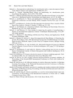
whereas leaves are denoted as triangles. Note that this decision tree incorporates
both nominal and numeric attributes. Given this classifier, the analyst can predict
the response of a potential customer (by sorting it down the tree), and understand
the behavioral characteristics of the entire potential customers population regarding
direct mailing. Each node is labeled with the attribute it tests, and its branches are
labeled with its corresponding values.
Age
Gender
Last R.
Yes
No
Yes
No
Yes
Female
male
NoNo
No
<=30
>30
Fig. 9.1. Decision Tree Presenting Response to Direct Mailing.
In case of numeric attributes, decision trees can be geometrically interpreted as
a collection of hyperplanes, each orthogonal to one of the axes. Naturally, decision-
makers prefer less complex decision trees, since they may be considered more com-
prehensible. Furthermore, according to Breiman et al. (1984) the tree complexity
has a crucial effect on its accuracy. The tree complexity is explicitly controlled by
the stopping criteria used and the pruning method employed. Usually the tree com-
plexity is measured by one of the following metrics: the total number of nodes, total
number of leaves, tree depth and number of attributes used. Decision tree induction
is closely related to rule induction. Each path from the root of a decision tree to one

of its leaves can be transformed into a rule simply by conjoining the tests along the
path to form the antecedent part, and taking the leaf’s class prediction as the class
9 Classification Trees 151
value. For example, one of the paths in Figure 9.1 can be transformed into the rule:
“If customer age is is less than or equal to or equal to 30, and the gender of the cus-
tomer is “Male” – then the customer will respond to the mail”. The resulting rule set
can then be simplified to improve its comprehensibility to a human user, and possibly
its accuracy (Quinlan, 1987).
9.2 Algorithmic Framework for Decision Trees
Decision tree inducers are algorithms that automatically construct a decision tree
from a given dataset. Typically the goal is to find the optimal decision tree by mini-
mizing the generalization error. However, other target functions can be also defined,
for instance, minimizing the number of nodes or minimizing the average depth.
Induction of an optimal decision tree from a given data is considered to be a
hard task. It has been shown that finding a minimal decision tree consistent with the
training set is NP–hard (Hancock et al., 1996). Moreover, it has been shown that
constructing a minimal binary tree with respect to the expected number of tests re-
quired for classifying an unseen instance is NP–complete (Hyafil and Rivest, 1976).
Even finding the minimal equivalent decision tree for a given decision tree (Zantema
and Bodlaender, 2000) or building the optimal decision tree from decision tables is
known to be NP–hard (Naumov, 1991).
The above results indicate that using optimal decision tree algorithms is feasible
only in small problems. Consequently, heuristics methods are required for solving
the problem. Roughly speaking, these methods can be divided into two groups: top–
down and bottom–up with clear preference in the literature to the first group.
There are various top–down decision trees inducers such as ID3 (Quinlan, 1986)!
C4.5 (Quinlan, 1993), CART (Breiman et al., 1984). Some consist of two conceptual
phases: growing and pruning (C4.5 and CART). Other inducers perform only the
growing phase.
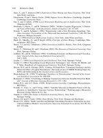
Figure 9.2 presents a typical algorithmic framework for top–down inducing of a

decision tree using growing and pruning. Note that these algorithms are greedy by
nature and construct the decision tree in a top–down, recursive manner (also known
as “divide and conquer“). In each iteration, the algorithm considers the partition of
the training set using the outcome of a discrete function of the input attributes. The
selection of the most appropriate function is made according to some splitting mea-
sures. After the selection of an appropriate split, each node further subdivides the
training set into smaller subsets, until no split gains sufficient splitting measure or a
stopping criteria is satisfied.
9.3 Univariate Splitting Criteria
9.3.1 Overview
In most of the cases, the discrete splitting functions are univariate. Univariate means
that an internal node is split according to the value of a single attribute. Consequently,
152 Lior Rokach and Oded Maimon
TreeGrowing (S,A,y,SplitCriterion,StoppingCriterion)
where:
S - Training Set
A - Input Feature Set
y - Target Feature
SplitCriterion - the method for evaluating a certain split
StoppingCriterion - the criteria to stop the growing process
Create a new tree T with a single root node.
IF StoppingCriterion(S) THEN
Mark T as a leaf with the most
common value of y in S as a label.
ELSE
Find attribute a that obtains the best SplitCriterion(a
i
,S).
Label t with a
FOR each outcome v

i
of a:
Set Subtree
i
= TreeGrowing (
σ
a=v
i
S,A,y).
Connect the root node of t
T
to Subtree
i
with
an edge that is labelled as v
i
END FOR
END IF RETURN TreePruning (S,T ,y)
TreePruning (S,T ,y)
Where: S - Training Set
y - Target Feature T - The tree to be pruned
DO
Select a node t in T such that pruning it
maximally improve some evaluation criteria
IF t =Ø THEN T = pruned(T,t)
UNTIL t = Ø
RETURN T
Fig. 9.2. Top-Down Algorithmic Framework for Decision Trees Induction.
the inducer searches for the best attribute upon which to split. There are various
univariate criteria. These criteria can be characterized in different ways, such as:

• According to the origin of the measure: information theory, dependence, and
distance.
• According to the measure structure: impurity based criteria, normalized impurity
based criteria and Binary criteria.
The following section describes the most common criteria in the literature.
9 Classification Trees 153
9.3.2 Impurity-based Criteria
Given a random variable x with k discrete values, distributed according to P =
(p
1
, p
2
, ,p
k
), an impurity measure is a function
φ
:[0, 1]
k
→ R that satisfies the
following conditions:
•
φ
(P)≥0
•
φ
(P) is minimum if ∃i such that component p
i
=1.
•
φ

(P) is maximum if ∀i, 1 ≤ i ≤ k, p
i
= 1/k.
•
φ
(P) is symmetric with respect to components of P.
•
φ
(P) is smooth (differentiable everywhere) in its range.
Note that if the probability vector has a component of 1 (the variable x gets only
one value), then the variable is defined as pure. On the other hand, if all components
are equal, the level of impurity reaches maximum.
Given a training set S, the probability vector of the target attribute y is defined as:
P
y
(S)=
⎛
⎝


σ
y=c
1
S


|
S
|
, ,




σ
y=c
|
dom(y)
|
S



|
S
|
⎞
⎠
The goodness–of–split due to discrete attribute a
i
is defined as reduction in impurity
of the target attribute after partitioning S according to the values v
i,j
∈ dom(a
i
):
ΔΦ
(a
i
,S)=
φ

(P
y
(S)) −
|
dom(a
i
)
|
∑
j=1
|
σ
a
i
=v
i, j
S|
|S|
·
φ
(P
y
(
σ
a
i
=v
i, j
S))
9.3.3 Information Gain

Information gain is an impurity-based criterion that uses the entropy measure (origin
from information theory) as the impurity measure (Quinlan, 1987).
In f ormationGain(a
i
,S)=
Entropy(y,S) −
∑
v
i, j
∈dom(a
i
)



σ
a
i
=v
i, j
S



|
S
|
·Entropy(y,
σ
a

i
=v
i, j
S)
where:
Entropy(y,S)=
∑
c
j
∈dom(y)
−


σ
y=c
j
S


|
S
|
·log
2


σ
y=c
j
S



|
S
|
9.3.4 Gini Index
Gini index is an impurity-based criterion that measures the divergences between the
probability distributions of the target attribute’s values. The Gini index has been used
in various works such as (Breiman et al., 1984) and (Gelfand et al., 1991) and it is
defined as:
154 Lior Rokach and Oded Maimon
Gini(y,S)=1 −
∑
c
j
∈dom(y)



σ
y=c
j
S


|
S
|

2

Consequently the evaluation criterion for selecting the attribute a
i
is defined as:
GiniGain(a
i
,S)=Gini(y,S) −
∑
v
i, j
∈dom(a
i
)


σ
a
i
=v
i, j
S


|
S
|
·Gini(y,
σ
a
i
=v

i, j
S)
9.3.5 Likelihood-Ratio Chi–Squared Statistics
The likelihood–ratio is defined as (Attneave, 1959)
G
2
(a
i
,S)=2 ·ln(2) ·
|
S
|
·In f ormationGain(a
i
,S)
This ratio is useful for measuring the statistical significance of the information gain
criterion. The zero hypothesis (H
0
) is that the input attribute and the target attribute
are conditionally independent. If H
0
holds, the test statistic is distributed as
χ
2
with
degrees of freedom equal to: (dom(a
i
) −1) ·(dom(y)−1).
9.3.6 DKM Criterion
The DKM criterion is an impurity-based splitting criterion designed for binary class

attributes (Dietterich et al., 1996) and (Kearns and Mansour, 1999). The impurity-
based function is defined as:
DKM(y,S)=2 ·







σ
y=c
1
S


|
S
|

·



σ
y=c
2
S



|
S
|

It has been theoretically proved (Kearns and Mansour, 1999) that this criterion
requires smaller trees for obtaining a certain error than other impurity based criteria
(information gain and Gini index).
9.3.7 Normalized Impurity Based Criteria
The impurity-based criterion described above is biased towards attributes with larger
domain values. Namely, it prefers input attributes with many values over attributes
with less values (Quinlan, 1986). For instance, an input attribute that represents the
national security number will probably get the highest information gain. However,
adding this attribute to a decision tree will result in a poor generalized accuracy. For
that reason, it is useful to “normalize” the impurity based measures, as described in
the following sections.
9 Classification Trees 155
9.3.8 Gain Ratio
The gain ratio “normalizes” the information gain as follows (Quinlan, 1993):
GainRatio(a
i
,S)=
In f ormationGain(a
i
,S)
Entropy(a
i
,S)
Note that this ratio is not defined when the denominator is zero. Also the ratio may
tend to favor attributes for which the denominator is very small. Consequently, it is
suggested in two stages. First the information gain is calculated for all attributes. As

a consequence, taking into consideration only attributes that have performed at least
as good as the average information gain, the attribute that has obtained the best ratio
gain is selected. It has been shown that the gain ratio tends to outperform simple
information gain criteria, both from the accuracy aspect, as well as from classifier
complexity aspects (Quinlan, 1988).
9.3.9 Distance Measure
The distance measure, like the gain ratio, normalizes the impurity measure. However,
it suggests normalizing it in a different way (Lopez de Mantras, 1991):
ΔΦ
(a
i
,S)
−
∑
v
i, j
∈dom(a
i
)
∑
c
k
∈dom(y)
|
σ
a
i
=v
i, j
AND y=c

k
S|
|S|
·log
2
|
σ
a
i
=v
i, j
AND y=c
k
S|
|S|
9.3.10 Binary Criteria
The binary criteria are used for creating binary decision trees. These measures are
based on division of the input attribute domain into two sub-domains.
Let
β
(a
i
,dom
1
(a
i
),dom
2
(a
i

),S) denote the binary criterion value for attribute a
i
over sample S when dom
1
(a
i
) and dom
2
(a
i
) are its corresponding subdomains. The
value obtained for the optimal division of the attribute domain into two mutually
exclusive and exhaustive sub-domains is used for comparing attributes.
9.3.11 Twoing Criterion
The gini index may encounter problems when the domain of the target attribute is
relatively wide (Breiman et al., 1984). In this case it is possible to employ binary
criterion called twoing criterion. This criterion is defined as:
twoing(a
i
,dom
1
(a
i
),dom
2
(a
i
),S)=
0.25 ·




σ
a
i
∈dom
1
(a
i
)
S



|
S
|
·



σ
a
i
∈dom
2
(a
i
)
S




|
S
|
·

∑
c
i
∈dom(y)








σ
a
i
∈dom
1
(a
i
) AND y=c
i
S







σ
a
i
∈dom
1
(a
i
)
S



−



σ
a
i
∈dom
2
(a
i
)AND y=c

i
S






σ
a
i
∈dom
2
(a
i
)
S









2
When the target attribute is binary, the gini and twoing criteria are equivalent. For
multi–class problems, the twoing criteria prefer attributes with evenly divided splits.
156 Lior Rokach and Oded Maimon

9.3.12 Orthogonal (ORT) Criterion
The ORT criterion was presented by Fayyad and Irani (1992). This binary criterion
is defined as:
ORT (a
i
,dom
1
(a
i
),dom
2
(a
i
),S)=1 −cos
θ
(P
y,1
,P
y,2
)
where
θ
(P
y,1
, P
y,2
) is the angle between two vectors P
y,1
and P
y,2

. These vectors rep-
resent the probability distribution of the target attribute in the partitions
σ
a
i
∈dom
1
(a
i
)
S
and
σ
a
i
∈dom
2
(a
i
)
S respectively.
It has been shown that this criterion performs better than the information gain
and the Gini index for specific problem constellations.
9.3.13 Kolmogorov–Smirnov Criterion
A binary criterion that uses Kolmogorov–Smirnov distance has been proposed in
Friedman (1977) and Rounds (1980). Assuming a binary target attribute, namely
dom(y)={c
1
,c
2

}, the criterion is defined as:
KS(a
i
,dom
1
(a
i
),dom
2
(a
i
),S)=







σ
a
i
∈dom
1
(a
i
) AND y=c
1
S





σ
y=c
1
S


−


σ
a
i
∈dom
1
(a
i
)AND y=c
2
S




σ
y=c
2
S








This measure was extended in (Utgoff and Clouse, 1996) to handle target at-
tributes with multiple classes and missing data values. Their results indicate that the
suggested method outperforms the gain ratio criteria.
9.3.14 AUC–Splitting Criteria
The idea of using the AUC metric as a splitting criterion was recently proposed
in (Ferri et al., 2002). The attribute that obtains the maximal area under the convex
hull of the ROC curve is selected. It has been shown that the AUC–based splitting
criterion outperforms other splitting criteria both with respect to classification ac-
curacy and area under the ROC curve. It is important to note that unlike impurity
criteria, this criterion does not perform a comparison between the impurity of the
parent node with the weighted impurity of the children after splitting.
9.3.15 Other Univariate Splitting Criteria
Additional univariate splitting criteria can be found in the literature, such as per-
mutation statistics (Li and Dubes, 1986), mean posterior improvements (Taylor and
Silverman, 1993) and hypergeometric distribution measures (Martin, 1997).
9 Classification Trees 157
9.3.16 Comparison of Univariate Splitting Criteria
Comparative studies of the splitting criteria described above, and others, have been
conducted by several researchers during the last thirty years, such as (Baker and
Jain, 1976, BenBassat, 1978, Mingers, 1989, Fayyad and Irani, 1992, Buntine and
Niblett, 1992, Loh and Shih, 1997, Loh and Shih, 1999, Lim et al., 2000). Most of
these comparisons are based on empirical results, although there are some theoretical
conclusions.

Many of the researchers point out that in most of the cases, the choice of split-
ting criteria will not make much difference on the tree performance. Each criterion
is superior in some cases and inferior in others, as the “No–Free–Lunch” theorem
suggests.
9.4 Multivariate Splitting Criteria
In multivariate splitting criteria, several attributes may participate in a single node
split test. Obviously, finding the best multivariate criteria is more complicated than
finding the best univariate split. Furthermore, although this type of criteria may dra-
matically improve the tree’s performance, these criteria are much less popular than
the univariate criteria.
Most of the multivariate splitting criteria are based on the linear combination of
the input attributes. Finding the best linear combination can be performed using a
greedy search (Breiman et al., 1984,Murthy, 1998), linear programming (Duda and
Hart, 1973,Bennett and Mangasarian, 1994), linear discriminant analysis (Duda and
Hart, 1973,Friedman, 1977,Sklansky and Wassel, 1981, Lin and Fu, 1983,Loh and
Vanichsetakul, 1988, John, 1996) and others (Utgoff, 1989a, Lubinsky, 1993, Sethi
and Yoo, 1994).
9.5 Stopping Criteria
The growing phase continues until a stopping criterion is triggered. The following
conditions are common stopping rules:
1. All instances in the training set belong to a single value of y.
2. The maximum tree depth has been reached.
3. The number of cases in the terminal node is less than the minimum number of
cases for parent nodes.
4. If the node were split, the number of cases in one or more child nodes would be
less than the minimum number of cases for child nodes.
5. The best splitting criteria is not greater than a certain threshold.
158 Lior Rokach and Oded Maimon
9.6 Pruning Methods
9.6.1 Overview

Employing tightly stopping criteria tends to create small and under–fitted decision
trees. On the other hand, using loosely stopping criteria tends to generate large de-
cision trees that are over–fitted to the training set. Pruning methods originally sug-
gested in (Breiman et al., 1984) were developed for solving this dilemma. According
to this methodology, a loosely stopping criterion is used, letting the decision tree to
overfit the training set. Then the over-fitted tree is cut back into a smaller tree by
removing sub–branches that are not contributing to the generalization accuracy. It
has been shown in various studies that employing pruning methods can improve the
generalization performance of a decision tree, especially in noisy domains.
Another key motivation of pruning is “trading accuracy for simplicity” as pre-
sented in (Bratko and Bohanec, 1994). When the goal is to produce a sufficiently
accurate compact concept description, pruning is highly useful. Within this process,
the initial decision tree is seen as a completely accurate one. Thus the accuracy of a
pruned decision tree indicates how close it is to the initial tree.
There are various techniques for pruning decision trees. Most of them perform
top-down or bottom-up traversal of the nodes. A node is pruned if this operation im-
proves a certain criteria. The following subsections describe the most popular tech-
niques.
9.6.2 Cost–Complexity Pruning
Cost-complexity pruning (also known as weakest link pruning or error-complexity
pruning) proceeds in two stages (Breiman et al., 1984). In the first stage, a sequence
of trees T
0
,T
1
, ,T
k
is built on the training data where T
0
is the original tree before

pruning and T
k
is the root tree.
In the second stage, one of these trees is chosen as the pruned tree, based on its
generalization error estimation.
The tree T
i+1
is obtained by replacing one or more of the sub–trees in the prede-
cessor tree T
i
with suitable leaves. The sub–trees that are pruned are those that obtain
the lowest increase in apparent error rate per pruned leaf:
α
=
ε
(pruned(T,t),S) −
ε
(T,S)
|
leaves(T )
|
−
|
leaves(pruned(T,t))
|
where
ε
(T,S) indicates the error rate of the tree T over the sample S and
|
leaves(T)

|
denotes the number of leaves in T. pruned(T,t) denotes the tree obtained by replacing
the node t in T with a suitable leaf.
In the second phase the generalization error of each pruned tree T
0
,T
1
, ,T
k
is
estimated. The best pruned tree is then selected. If the given dataset is large enough,
the authors suggest breaking it into a training set and a pruning set. The trees are
constructed using the training set and evaluated on the pruning set. On the other
hand, if the given dataset is not large enough, they propose to use cross–validation
methodology, despite the computational complexity implications.
9 Classification Trees 159
9.6.3 Reduced Error Pruning
A simple procedure for pruning decision trees, known as reduced error pruning, has
been suggested by Quinlan (1987). While traversing over the internal nodes from the
bottom to the top, the procedure checks for each internal node, whether replacing
it with the most frequent class does not reduce the tree’s accuracy. In this case, the
node is pruned. The procedure continues until any further pruning would decrease
the accuracy.
In order to estimate the accuracy, Quinlan (1987) proposes to use a pruning set.
It can be shown that this procedure ends with the smallest accurate sub–tree with
respect to a given pruning set.
9.6.4 Minimum Error Pruning (MEP)
The minimum error pruning has been proposed in (Olaru and Wehenkel, 2003). It
performs bottom–up traversal of the internal nodes. In each node it compares the
l-probability error rate estimation with and without pruning.

The l-probability error rate estimation is a correction to the simple probability
estimation using frequencies. If S
t
denotes the instances that have reached a leaf t,
then the expected error rate in this leaf is:
ε

(t)=1 − max
c
i
∈dom(y)


σ
y=c
i
S
t


+ l · p
apr
(y = c
i
)
|
S
t
|
+ l

where p
apr
(y = c
i
) is the a–priori probability of y getting the value c
i
, and l
denotes the weight given to the a–priori probability.
The error rate of an internal node is the weighted average of the error rate of its
branches. The weight is determined according to the proportion of instances along
each branch. The calculation is performed recursively up to the leaves.
If an internal node is pruned, then it becomes a leaf and its error rate is calculated
directly using the last equation. Consequently, we can compare the error rate before
and after pruning a certain internal node. If pruning this node does not increase the
error rate, the pruning should be accepted.
9.6.5 Pessimistic Pruning
Pessimistic pruning avoids the need of pruning set or cross validation and uses the
pessimistic statistical correlation test instead (Quinlan, 1993).
The basic idea is that the error ratio estimated using the training set is not reliable
enough. Instead, a more realistic measure, known as the continuity correction for
binomial distribution, should be used:
ε

(T, S)=
ε
(T,S)+
|
leaves(T )
|
2 ·

|
S
|