96 Introduction and Background
is discussed based on experimental observations of the type that are classified as all-or-
nothing or quantal. While it is generally desirable to have quantitative measurements,
many cases can be expressed only as “occurring” or “not-occurring.” The obvious example
with insects is death. The analogous situation with FLSs, especially those obtained from
staircase type testing, is failure or survival (run-outs) after a certain number of cycles.
Not only is it important to analyze the data, but the planning of the experiments is equally
important. The type of fatigue testing carried out, for example, the number of tests at each
of several stress levels, can influence the results. In the application of statistical methods
to biological data, Fisher [37] suggested that the statistician should be consulted during
the planning of an experiment and not only when statistical analysis of the results is
required. His advice on experimental design may greatly increase the value of the results
eventually obtained, whether they be biological experiments or FLS experiments.
For the staircase method, we can determine the average fatigue limit, 
sc
, and its
standard deviation, 
sc
, from the equations of Dixon and Mood [35], which are also
presented in an ASTM publication [38].
∗
The method is based on a maximum-likelihood
estimation (MLE) and provides approximate formulas to calculate the mean and standard
deviation, assuming that the FLS follows a Gaussian (normal) distribution. The equations
for the mean and standard deviation are

sc
=S
i =0
+s
⎛

⎜
⎜
⎝
i
max

i =0
im
i
i
max

i =0
m
i
± 05
⎞
⎟
⎟
⎠
(3.2)

sc
=162 s
⎛
⎜
⎜
⎜
⎝
i

max

i =0
m
i
i
max

i =0
i
2
m
i
−

i
max

i =0
im
i

2

i
max

i =0
m
i


2
+0029
⎞
⎟
⎟
⎟
⎠
(3.3)
provided
i
max

i =0
m
i
i
max

i =0
i
2
m
i
−

i
max

i =0

im
i

2

i
max

i =0
m
i

2
> 03 (3.4)
When the quantity above is ≤ 0 3, the mathematics becomes very complicated and a
rough approximation can be made using 
sc
= 053 s [35]. In the above equations, s is
the step size, the parameter “ i ” is an integer that denotes the stress level and i
max
is the
∗
The subscript “sc” refers to staircase tests. In statistics,  and  are commonly used to represent the mean
and standard deviation, respectively. The latter often causes confusion because  is used to represent stress in
the field of solid mechanics.
Accelerated Test Techniques 97
highest level in the staircase, while m
i
is the number of broken or non-broken specimens
at level i, depending upon whether or not most of the specimens are non-broken or broken,

respectively. If most of the specimens have broken, i =0 corresponds to the lowest step
at which a specimen survives. On the other hand, if most of the specimens survive, i =0
is the lowest stress at which a specimen fails. The plus sign in Equation (3.2) is used
when the analysis is based on the survivals, and the minus sign when it is based on the
failures. This rule is often stated incorrectly in the literature (see [34, 35], for example) or
not addressed at all (see [39], for example). It is somewhat confusing because if failure
is the more common event, then the analysis is based on the number of survivals. Thus,
it should be stated (correctly) that the plus sign is used when the more frequent event is
failure, and the minus sign is used when the more frequent event is survival. In the case
where equal numbers of specimens fail or survive, either calculation provides the same
result as would be expected. Of significance is the observation that the computations are
based on the incidence and values of the less frequent event, failure or survival.
Some examples of the application of the analysis of the distribution function for some
specific data sets are given here. The data of Epremian and Mehl, Figures 3.23 and 3.24,
Ransom and Mehl, Figures 3.25 and 3.26, and titanium from the National High Cycle
Fatigue program, Figures 3.27 and 3.28, are summarized in Table 3.1.
The calculated values for the mean stress, shown in the table, agree reasonably well
with those shown in the probability plots, Figures 3.24, 3.26, and 3.28, since both are
based on an assumption of a normal distribution function for the FLS. The first series of
tests, those of Epremian and Mehl, represent the largest number of tests of the three being
evaluated, and show the best fit to a normal distribution curve in Figures 3.23 and 3.24,
and the lowest ratio of the standard deviation, s, to the mean as shown in the last column
of Table 3.1. The data of Ransom and Mehl, on the other hand, show little resemblance
to a normal distribution function, Figures 3.25 and 3.26, yet the calculation for the ratio
of the standard deviation to the mean shows this ratio not to be that large. The third set
of data on titanium represents the fewest number of staircase tests, shows a reasonable
fit to a standard deviation, but indicates a very high degree of dispersion. The dispersion
appears to be more a function of the number of tests than the true inherent dispersion of
the material property (FLS) being evaluated.
Another application of the staircase method is illustrated in [40] where, for each

of 3 mean shear stresses, the alternating shear stress for a fatigue limit corresponding
Table 3.1. Summary of statistical evaluations using Dixon and Mood method
Reference # fail # survive 
sc
(ksi) 
sc
(ksi) /mean
Epremian and Mehl 93 43 40.96 1.43 1.15
Ransom and Mehl 27 27 46.27 2.93 1.29
National HCF Ti 12 14 78.0 8.95 1.60
98 Introduction and Background
to 5×10
6
cycles (run-out) was desired. Thirteen specimens were tested at each mean stress
(0, 45, and 90 MPa) using a shear stress increment of 15 MPa. With the limited number
of specimens (13) tested at each mean stress level, the calculated standard deviation
was determined to not be statistically significant because of the small number of tests.
It is of significance to note that the standard deviation was found to be less than the
stress increment of 15 MPa. Using the assumption that the fatigue limit follows a normal
distribution, the authors concluded that there were not enough samples tested to compare
the fatigue limit as a function of mean stress in a statistically significant manner.
Data from fatigue strength tests, where the result of any single test is either fail or
survive before a specific number of cycles at the given stress level (S) of the test, can
be plotted in terms of the proportions failed (P), the number failed divided by the total
number tested at that stress level. The fatigue strength data can be obtained from either
testing equal numbers of specimens at equally spaced stress levels ( P–S tests) or from
up-and-down (staircase) testing, described above, where the majority of tests end up at
stresses near the median fatigue strength at the specific number of cycles. The up-and-
down testing can be used to precede the P–S tests, or to generate design data. But it has
been pointed out that the insoluble problem in strength analyses is to establish the true

shape of the underlying strength distribution function [41]. If only the median strength
is desired, then it makes little difference which distribution function is used in analysis
of the data. On the other hand, if the tails or the spread of the distribution function
are needed for design, for example, then the results are very sensitive to the form of
the actual distribution function. Another advantage of the up-and-down method is that
small sample numbers can be used to accurately determine the median strength [41].
Regardless of the analysis involved, there are basically two forms of plots which display
quantal response data (fail or survive), one having a linear scale for P and one where P
is plotted on probability paper. Such plots were shown, for example, in Figures 3.23 and
3.24, above.
The primary requirement for the use of the simple statistical analysis of the results from
staircase testing is that the variate under analysis be normally (Gaussian) distributed. If
not, the natural variate can be transformed to one that does have a normal distribution. The
logarithm of the natural variate is often used. While the staircase method is particularly
effective in estimating the mean, it is not a good method for estimating the extremes of
the distribution unless normality of the distribution can be assured. A second condition
is that the sample size be large if the analysis is to be applicable since it is based
on large sample theory. A third condition requires that the standard deviation must be
larger than the interval of the variate in the staircase testing procedure, a condition that
is not generally known before the testing begins. A more desirable situation is if the
interval used is less than twice the standard deviation [35]. Lin et al. [34] recommend
that the fixed stress increment should be in the range from half to twice the standard
deviation.
Accelerated Test Techniques 99
3.4.2.2. Numerical simulations
To further demonstrate some of the statistical aspects of the staircase test procedure,
numerical simulations have been conducted. The FLS is assumed to be distributed nor-
mally. A hypothetical material having a median FLS of 50 and a standard deviation of
5 was chosen. The mean value is an arbitrary unit for this material, only the standard
deviation, s, is of importance in the numerical examples.

The first numerical exercise consisted of simulating a series of staircase tests using
different numbers of samples, ranging from 10 to 50, and different step sizes, ranging
from 01s to 10s, where s is the standard deviation (5 in this case). For each test
simulation, a random number for the FLS was generated from EXCEL corresponding to a
normal distribution with the mean of 50 and s =5. The protocol for the staircase test was
followed numerically, but the first test of each series was started at the mean value of 50.
For each different value of the stress increment, the same set of random numbers for the
FLS was used for each set of numbers of tests. The results are summarized in Table 3.2.
The results are not statistically very significant since only one simulation was conducted
for each condition. Nonetheless, the values for the standard deviation obtained from the
formulas of Dixon and Mood [35] show no trend or relationship to the “true” distribution
where a value of s = 5 was chosen. On the other hand, the values for the mean FLS,
which was chosen as 50 in the simulation, are reasonably close for all of the conditions
simulated. While little can be stated about the significance of these results, the trend
for a better value (closer to 50) with larger number of tests and decreasing size of the
increment between each successive test simulation in the staircase procedure seems to
be established, although very weakly. From these results, it would be recommended that
the fixed stress increment would ideally be less than half of the standard deviation which
is a much tighter guideline that either those of Dixon and Mood [35] or, more recently,
Lin et al. [34].
To further explore the trend with number of tests, the numerical exercises were repeated
10 times each for numbers of tests of 10, 30, and 50. The random numbers for each value
of the FLS were chosen corresponding to the same normal distribution as above, with
Table 3.2. Normal distribution, mean =50s= standard deviation
Increment 0.1 s 0.25 s 0.5 s 1.0 s
# trials Mean s Mean s Mean s Mean s
10 51.58 5.60 51.50 3.29 52.25 2.71 52.50 6.71
20 50.86 2.50 50.50 1.67 51.25 4.17 53.50 4.77
30 50.68 0.70 51.03 1.53 50.92 1.67 51.50 2.61
40 50.39 5.23 48.50 10.62 47.75 5.95 49.00 7.61

50 50.83 6.48 50.71 3.82 50.55 3.53 50.70 5.34
100 Introduction and Background
Table 3.3. Mean = 50 increment =05 01s mean = 50
# Tests 10 30 50
Trial # Mean s Mean s Mean s
1 49.85 0.48 49.79 1.23 50.61 0.77
2 48.13 0.58 51.63 2.20 51.82 2.70
3 49.35 0.48 49.04 1.15 51.92 6.53
4 48.75 1.64 49.32 1.28 49.81 2.25
5 50.42 0.74 49.65 0.59 51.23 4.92
6 51.92 0.74 51.13 1.54 49.94 1.97
7 49.35 0.48 50.75 0.49 50.48 3.33
8 50.05 0.54 50.12 0.83 49.73 2.97
9 48.85 1.13 48.93 2.06 50.97 1.49
10 50.00 0.23 49.46 1.84 50.57 6.37
Mean 49.67 0.70 49.98 1.32 50.71 3.33
Std Dev 1.05 0.91 0.78
mean = 50 and s = 5. All of the simulations corresponded to staircase tests that started
with a value of 50 for the first test and used a FLS increment of 0.5 which corresponds
to 0.1s. The results of each test series simulation are summarized in Table 3.3. For the 10
test series simulated for totals of 10, 30, or 50 tests in each series, the mean value and the
standard deviation is computed at the bottom of the table. Statisticians will recommend
that up to 100 trials should be performed before the results start to be statistically
significant, but the results of 10 trials show the trends adequately. For FLS increments
corresponding to 01s, reasonably accurate values of the mean value can be obtained from
as few as 10 tests in a staircase sequence, and more consistency is noted as the number
of tests is increased to 30 and to 50. In fact, looking at the numbers from these randomly
generated values of FLS for the simulations, the series of 50 tests provides numerical
values of the FLS that appear to be no better than those obtained from test series where
only 10 tests were simulated. From this, it appears that very large numbers of tests are

not needed to get a good approximation for the mean value when the increment between
tests is small and the starting value is near the correct value. Values for the standard
deviation of the distribution function of the value of FLS, however, do not provide any
consistent numbers related to the real distribution, even for as many as 50 tests in a test
sequence. As pointed out often in the literature, the staircase method concentrates testing
near the mean value and provides very little information about behavior at values of FLS
away from the mean.
The last part of these numerical simulations explored the consequences of starting the
simulated test series at values of FLS that were not at the “correct” value. For additional
simulations, the series of 50 tests shown in Table 3.3 was duplicated, using the same
statistical distribution of values for FLS, but the starting values for the first test were
Accelerated Test Techniques 101
Table 3.4. All tests at inc =05 01s Mean =5050 tests
Start value 45 55 50
Trial # Mean s Mean s Mean s
14998 152 5075 301 5061 0.77
24853 544 5266 190 5182 2.70
35056 1419 5275 131 5192 6.53
44973 581 5038 277 4981 2.25
55047 1480 5255 353 5123 4.92
64963 403 5101 619 4994 1.97
74918 606 5138 1058 5048 3.33
84960 643 5060 432 4973 2.97
94961 659 5272 220 5097 1.49
10 50
08 815 5113 998 5057 6.37
Mean 4974 730 5159 458 5071 3.33
Std Dev 060 097 078
chosen as either 45 or 55. These values are an amount “s” away from the true value
of 50. Computed values for the mean and standard deviation for these starting values

in each test series simulation, along with the baseline using a starting value of 50, are
shown in Table 3.4. The simulation for a starting value of 50 is repeated from Table 3.3,
and the same 50 random numbers for FLS were used for each starting value. The results
are summarized in Table 3.4 which shows that values for the mean FLS do not appear to
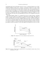
be dependent on the starting value of the test series. To further illustrate what happens
in a series of staircase tests such as these, the results for the last trial (#10) are presented
graphically in Figure 3.29. In this figure, the sequence of testing is illustrated on a test-
by-test basis for each of the 3 starting values of FLS, 45, 55, and 50. What the figure
illustrates is that starting low or high with respect to the mean requires a number of tests
before the tests start oscillating about the mean as the staircase method proceeds. In the
series of 50 tests, the data from a single simulation show that between 10 and 20 tests
are required before the staircase method approaches equilibrium. What this produces,
in essence, is a smaller test sequence. So although 50 tests are conducted, the results
correspond to a test sequence of only 30 to 40 tests. In the particular case illustrated, it is
not before the 19th test that the stresses at which the tests are conducted are within one
unit of each other, and at the 28th test the tests are identical. Recall that the randomly
generated numerical values for each of the three simulations are identical and occur in
the same order. Thus, after the 28th test in each simulation, the three plots in Figure 3.29
are identical.
Further work on numerical simulations of the staircase method has been conducted
as part of a PhD dissertation by Major Randall Pollak at the Air Force Institute of
Technology. The results of these extensive simulations as well as some suggestions for
102 Introduction and Background
40
45
50
55
60
01020304050
Failure

Survive
Value of FLS
Specimen number
FLS
0
= 50.08
Normal distribution
Mean = 50
Std dev = 5
Start at 45
0.5 increments
(a)
40
45
50
55
60
Failure
Survive
Value of FLS
Specimen number
FLS
0

=

51.13
Normal distribution
Mean


=

50
Std dev

=

5
Start at 55
0.5 increments
(b)
0
10
20 30 40 50
Normal distribution
Mean
= 50
Std dev
= 5
Start at 50
0.5 increments
40
45
50
55
60
Failure
Survive
Value of FLS
Specimen number

FLS
0
=

50.57
(c)
0 1020304050
Figure 3.29. Illustration of numerical simulation of staircase tests for different starting values of FLS.
(a) FLS =45; (b) FLS = 55; (c) FLS = 50.
Accelerated Test Techniques 103
optimizing the test procedure to determine the FLS at a large number of cycles are
presented in Appendix D. These simulations produce somewhat different guidance than
that reported previously in the literature as described above. Of greatest significance is
the finding that step sizes of the order of 17 are best for reducing standard deviation
bias, in contrast to the generally accepted guidance of using steps from 2/3to3/2.
The numerical simulations presented herein serve to illustrate the inherent weakness
of the staircase method, namely that good results can be very dependent on a knowledge
of the answer first, both for the mean value of FLS as well as the variance. Having this
information available in advance, such as from extrapolated LCF test data, will help in
choosing a starting value as well as a stress increment. If the starting value is low, many
tests will produce survival (run-out), so equilibrium about the mean value will not be
achieved right away. For such a sequence, the number of survivals will generally exceed
the number of failures. In the analysis, however, only the failed tests are counted. This,
in turn, has the net effect of having conducted fewer tests. The opposite is true when the
starting value is high compared to the actual mean. In either case, fewer effective tests are
performed, but the simulations shown above indicate that this does not seriously hamper
the ability to determine the mean value of the FLS from staircase tests.
For comparison to the statistical aspects of staircase testing, numerical simulations were
carried out to evaluate the statistical aspects of step testing. In this case, the assumption
will be made that a step test will provide a true value of the FLS and that no history

effects such as coaxing are present. This assumption has certainly not been proven in the
general case for all test conditions like number of steps and step sizes and for all materials.
Nonetheless, the numerical simulations are carried out assuming the FLS corresponding
to a specified number of cycles such as 10
7
follows a normal (Gaussian) distribution.
As in the above simulations for the staircase tests, the mean = 50 and the standard
deviation =5. These simulations amount to nothing more than a numerical evaluation of
how many samples have to be obtained to recover the properties of the normal distribution
if each sample follows that distribution function statistically. This type of information
is widely available in the statistics literature but is repeated here for comparison of test
methods for determining the FLS. The simulations were carried out assuming that the
number of step-test experiments conducted was either 10, 20, 30, 40, or 50. In the first
series of simulations, the procedure was repeated 10 times. This is essentially a test of the
randomness of a random number generator when the number of tests is finite. The results
of the simulations are presented in Table 3.5. For each number of experiments, the mean
and standard deviation of the 10 simulations are shown in columns 2 and 3. The standard
deviation of these quantities is shown in columns 4 and 5, respectively. This provides a
measure of the repeatability of the results of a single simulation. To get a better feel for
how random the numbers are, the same simulations were carried out 100 times and the
results are presented in Table 3.6. The simulations appear to be quite similar, but these
results give a slightly better feel for how accurately a normal distribution of values for
104 Introduction and Background
Table 3.5. Summary of numerical simulations of step tests repeated 10 times
# of Experiments Mean Std dev Std dev of mean Std dev of std dev
10 49.18 4.78 2.20 0.89
20 50.14 4.93 2.15 0.59
30 49.82 4.72 0.77 0.52
40 49.96 4.98 0.73 0.41
50 50.09 5.05 1.00 0.45

Table 3.6. Summary of numerical simulations of step tests repeated 100 times
# of Experiments Mean Std dev Std dev of mean Std dev of std dev
10 49.93 4.82 1.70 1.18
20 50.01 4.87 1.20 0.76
30 49.93 4.92 0.91 0.60
40 50.02 4.89 0.79 0.53
50 50.02 4.97 0.79 0.46
FLS can be expected to be reproduced from a finite number of test results. It can be seen
from the table that even for as few step tests as 10, the mean and standard deviation for
the FLS are close to the actual values, unlike the results shown earlier for the staircase
method. Thus, the type of information required from a test series (mean or scatter) should
help govern the type of test chosen.
3.4.2.3. Sample size considerations
The staircase method, or up-and-down method, was not originally explored for small
sample sizes in terms of the efficiency of the test method. In their original work, Dixon
and Mood [35] were concerned that “measures of reliability may well be very misleading
if the sample size is less than forty.” The numerical examples above seem to validate
that fear if looking for the standard deviation as well as the mean using the estimating
formulas from the original paper. Subsequent to their original work, the use of small
sample sizes was investigated by Brownlee et al. [42] and again by Dixon [43], among
others. Brownlee et al. [42] determined actual performance estimates for the mean based
on series of length 10 or less. They found that the Dixon and Mood formula for the
(asymptotic) variance is reasonably reliable even in samples as small as 5–10. They also
showed that the up-and-down method does not necessarily have to be run sequentially,
but might be run in a number of parallel short series without much loss of accuracy. Dixon
[43] developed a modified version of the original up-and-down method for small sample
sizes using sequentially determined test levels and sequentially determined sample sizes.
He provided tables from which estimates of the mean square error could be obtained and
Accelerated Test Techniques 105
showed that the error for the mean was relatively independent of the starting level of

the test sequence and the spacing between test levels. The procedure allows a design of
experiments approach where very small sample sizes can be achieved without sacrificing
accuracy.
The staircase method is the commonly used method for determining the statistical
characteristics of the fatigue strength at any specified life and is used in standards of the
British, Japanese, and French.
Staircase testing can be very expensive because of the large sample sizes and the
lengthy time at least for the survival tests which can be 10
7
cycles or longer, and comprise
approximately half of the staircase tests. Because of this, accelerated tests have been
proposed [34] where the HCF strength (e.g. at 10
7
cycles) is extrapolated from small
numbers of LCF (e.g. 10
3
–10
6
cycles). Doing this, however, requires an assumption of
the shape of the S–N curve over the LCF range and up to the HCF limit. In their work,
Lin et al. [34] assume an expression of the form
S
a
=S

f
N
f

b

(3.5)
where S
a
and N
f
represent the stress amplitude and number of cycles to failure, respec-
tively, and S

f
(fatigue strength coefficient) and b (fatigue strength exponent) are material
parameters fit to the data. In the methods used in [34], assumptions are made regarding
the statistical nature of the LCF data and its relation to the statistical fatigue limit strength
distribution.
3.4.2.4. Construction of an “artificial” staircase
There are times when conducting an entire staircase sequence is impractical and overly
time consuming. Perhaps it was not the initial objective when planning the experiments,
or some data already exist on S–N behavior at equal stress increments near the fatigue
limit. Rather than throwing out existing data, these data may be used and supplemented
by additional data to construct what will be called an “artificial” staircase. Recall that
for a “true” staircase, each subsequent test is conducted at a fixed stress increment either
above or below the previous stress level depending on whether the previous test resulted
in a survival or a failure, respectively, within the targeted number of cycles. If a batch
of data have been obtained at equally spaced stress levels, these data can be pooled
together and drawn from the pool in a random fashion, a method that is referred to as
the bootstrap method [44]. All of the data should be used, and no single data point may
be used more than once in constructing an artificial staircase sequence. Additional test
data may be required, at lower stresses if the majority of the data are failures, or at
higher stresses if most of the data are survivals. The mathematics of constructing such an
artificial sequence has not been developed, not is any analysis available to demonstrate