Alpert/Handbook of Algorithms for Physical Design Automation AU7242_C005 Finals Page 82 23-9-2008 #11
82 Handbook of Algorithms for Physical Design Automation
For each edge (u,v) ∈ E
If L[v] > L[u] + weight(uv)
Return: Negative Weighted Cycle Exists
The all pair shortest path problem tries to find the shortest paths between all vertices. Of course,
one approach is to execute the single-source shortest path algorithm for all the nodes. Much faster
algorithms like Floyd Warshall algorithm, etc. have also been developed.
5.5 NETWORK FLOW METHODS
Definition 5 A network is a directed graph G = (V , E) where each edge (u, v) ∈ E has a capacity
c(u, v) ≥ 0. There exists a node/vertex called the source, s and a destination/sink node, t. If an edge
does not exist in the network then its capacity is set to zero.
Definition 6 A flow in the network G is a real value function f : VXV → R. This has the following
properties:
1. Capacity constraint: Flow f (u, v) ≤ c(u, v) ∀ u, v ∈ V
2. Flow conservation: ∀ u ∈ V −{s, t}, 
v∈v
f (u, v) = 0
3. Skew symmetry: ∀ u, v ∈ V ,f (u, v) =−f (v, u)
The value of a flow is typically defined as the amount of flow coming out of the source to all
the other nodes in the network. It can equivalently be defined as the amount of flow coming into the
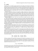
sink from all the other nodes in the network. Figure 5.4 illustrates an example of network flow.
Definition 7 Maximum flow problem is defined as the problem of finding a flow assignment to
the network such that it has the maximum value (note that a flow assignment must conform to the
flow properties as outlined above).
Network flow [4] fo rmulations have large applicability in various practical problems including
supply chain management, airline industry, and many others. Several VLSI CAD applications like
low power resource binding, etc. can be modeled as instances of network flow problems. Network
flow has also been applied in physical synthesis and design problems like buffer insertion.
Next, an algorithm is presented that solves the maximum flow problem optimally. This algorithm
was developed by Ford and Fulkerson. This is an iterative approach and starts with f (u, v) = 0for

Source: s
Cap
= 1
Cap
= 1 Cap = 1
Cap
= 1
Cap
= 2
Cap
= 2
Destination: t
Flow
= 1
Flow
= 1
Flow
= 1
Flow
= 1
Flow
= 1
Flow
= 0
FIGURE 5.4 Network flow.
Alpert/Handbook of Algorithms for Physical Design Automation AU7242_C005 Finals Page 83 23-9-2008 #12
Basic Algorithmic Techniques 83
all vertex pairs (u, v). At each step/iteratio n, the algorithm finds a path from s to t that still has
available capacity (this is a very simple explanation of a more complicated concept) and augments
more flow along it. Such a path is therefore called the augmenting path. This process is repeated till

no augmenting paths are found. The basic structure of the algorithm is as follows:
Ford-Fulkerson (G,s,t)
For each vertex pair (u,v)
f(u,v) = 0
While there is an augmenting path p from s to t
Send more flow along this path without violating
the capacity of any edge
Return f
At any iteration, augmenting path is no t simply a path of finite positive capacity in the graph.
Note that capacity of a path is defined by the capacity of the minimum capacity edge in the path. To
find an augmenting path, at a given iteration, a new graph called the residual graph is initialized. Let
us suppose that at a given iteration all vertex pairs uv have a flow of f (u, v). The residual capacity is
defined as follows:
c
f
(u, v) = c(uv) − f (u, v)
Note that the flow must never violate the capacity constraint. Conceptually, residual capacity is
the amount of extra flow we can send from u to v. A residual graph G
f
is defined as follows:
G
f
= (V, E
f
) where E
f
={(u, v), ∈ VXV: c
f
(u, v)>0}
The Ford Fulkerson method finds a path from s to t in this residual graph and sends more flow

along it as long as the capacity constraint is not violated. The run-time complexity of Ford Fulkerson
method is O(E
∗
f
max
) where E is the number of edges and f
max
is the value of the maximum flow.
Theorem 1 Maximum Flow Minimum Cut: If f is a flow in the network then the following
conditions are equivalent
1. f is the maximum flow
2. Residual network contains no augmenting paths
3. There exists a cut in the network with capacity equal to the flow f
A cut in a n etwork is a p artitioning of the nodes into two: with the source s on one side and
the sink t on another. The capacity of a cut is the sum of the capacity of all edges that start in the s
partition and end in the t partition.
There are several g eneralizations/extensions to the concept of maximum flow presented above.
Multiple sources and sinks: Handling multiple sources and sinks can be done easily. A super source
and a super sink node can be initialized. Infinite capacity edges can then be added from super source
to all the sources. Infinite capacity edges can also be added from all the sinks to the super sink.
Solving the maximum flow problem on this modified network is similar to solving it on the original
network.
Mincost flow: Mincost flow problems are of the following type. Assuming we need to pay a price for
sending each unit of flow o n an edge in the network. Given the cost per unit flow for all edges in the
network, we would like to send the maximum flow in such a way that it incurs the minimum total
Alpert/Handbook of Algorithms for Physical Design Automation AU7242_C005 Finals Page 84 23-9-2008 #13
84 Handbook of Algorithms for Physical Design Automation
cost. Modifications to the Ford Fulkerson method can be used to solve the mincost flow problem
optimally.
Multicommodity flow: So far the discussion has focused on just one type of flow. Several times many

commodities need to be transported on a network of finite edge capacities. The sharing of the same
network binds these commodities together.
These different commo dities represent different types of flow. A version of the multicommodity
problem could be described as follows. Given a network with nodes and edge capacities/costs,
multiple sinks and sources of different types of flow, satisfy the demands at all the sinks while
meeting the capacity constraint and with the minimum total cost. The multicommodity flow problem
is NP-complete and has been an active topic of research in the last few decades.
5.6 THEORY OF NP-COMPLETENESS
For algorithms to be computationally practical, it is typically desired that their order of complexity
be polynomial in the size of the problem. Problems like sorting, shortest path, etc. are examples for
which there exist algorithms of polynomial complexity. A natural question to ask is “Does there
exist a polynomial complexity algorithm for all problems?”. Certainly, the answer to this question is
no because there exist problems like halting problem that has been proven to not have an algorithm
(much less a polynomial time algorithm). NP-complete [3] problems are the ones for which we do
not know, as yet, if there exists a polynomial complexity algorithm. Typically, the set of all problems
that are solvable in polynomial time is called P. Before moving further, we would like to state that
the concept of P or NP-complete is typically developed around problems for which the solution is
either yes or no, a.k.a., decision problems. For example, the decision version for the maximum flow
problem could be “Given a network with finite edge capacities, a source, and a sink, can we send at
least K units of flow in the network?” One way to answer this question could be to simply solve the
maximum flow problem and check if it is greater than K or not.
Polynomial time verifiability : Let us suppose an oracle gives us the solution to a decision problem. If
there exists a polynomial time algorithm to validate if the answer to the decision problem is yes or no
for that solution, then the problem is polynomially verifiable. For example, in the decision version
of the maximum flow problem, if an oracle gives a flow solution, we can easily (in polynomial time)
check if the flow is more than K (yes)orlessthanK (no). Therefore, the decision version of the
maximum flow problem is polynomially verifiable.
NP class of problems: The problems in the set NP are verifiable in polynomial time. It is trivial to
show that all problems in the set P (all decision problems that are solvable in polynomial time) are
verifiable in polynomial time. Therefore, P ⊆ NP. But as of now it is unknown whether P = NP.

NP-complete problems: They have two characteristics:
1. Problems can be verified in polynomial time.
2. These problems can be transformed into one another using a polynomial number of steps.
Therefore, if there exists a polynomial time algorithm to solve any of the problems in this set,
each and every problem in the set becomes polynomially solvable. It just so happens that to date
nobody has been able to solve any of the problems in this set in polynomial time. Following is an
procedure for proving that a given decision problem is NP-complete:
1. Check whether the problem is in NP (polynomially verifiable).
2. Select a known NP-complete problem.
3. Transform this problem in polynomial steps to an instance of the pertinent problem.
4. Illustrate that given a solution to the known NP-complete problem, we can find a solution
to the pertinent problem and v ice versa.
Alpert/Handbook of Algorithms for Physical Design Automation AU7242_C005 Finals Page 85 23-9-2008 #14
Basic Algorithmic Techniques 85
If these conditions are satisfied by a g iven problem then it belongs to the set of NP-complete
problems.
The first problem to be proved NP-complete was Satisfiability or SAT by Stephen Cook in his
famous 1971 paper “The complexity of theorem proving procedures,” in Proceedings of the 3rd
Annual ACM Symposium on Theory of Computing. Shortly after the classic paper by Cook, Richard
Karp proved several other problems to be NP-complete. Since then the set of NP-complete problems
has been expanding. Several problems in VLSI CAD including technology mapping on DAGs, gate
duplication on DAGs, etc. are NP-complete.
E
XAMPLE
Illustrative Example: NP-Completeness of 3SAT
3SAT: Given a set of m clauses anded together F = C
1
·C
2
·C

3
·····C
m
. Each clause C
i
is a logical
OR of at most three boolean literals C
i
= (a + b +¯o) where ¯o is the negative phase of boolean variable
o. Does there exist an assignment of 0 /1 to each variable such that F evaluates to 1? (Note that this is a
decision problem.)
Proof of NP-Completeness: Given an assignment of 0/1 to the variables, we can see if each clause eval-
uates to 1.Ifall clausesevaluateto 1then F evaluates to 1else it is 0. This is asimple polynomial time algo-
rithm for verifying the decision giv en a specific solution or assignment of 0/1 to the variables. Therefore,
3SAT is in NP. Now let us transform the well-known NP-complete problem SAT to a n instance of 3SAT.
SAT: Given a set of m clauses anded together G = C
1
· C
2
· C
3
·····C
m
. Each clause C
i
is a logical
OR of boolean literals C
i
= (a +b +¯o + e + f +···). Does there exist an assignment of 0/1 to each
variable such that G evaluates to 1. (Note that this is a decision problem.)

To perform this tranformation, we look at each clause C
i
in the SAT problem with more than three
literals. LetC
i
= (x
1
+x
2
+x
3
+···+x
k
). This clause is replaced by k−2 new clauses eachwith length 3.
For this to happen, we introduce k −3newvariablesu
i
, , u
k−3
. These clauses are constructed as follows.
P
i
= (x
1
+ x
2
+u
1
)(x
3
+¯u

1
+ u
2
)(x
4
+¯u
2
+ u
3
)(x
5
+¯u
3
+ u
4
) ···(x
k−1
+ x
k
+¯u
k−3
)
Note that if there exists an assignment of 0/1 to x
1
, , x
k
for which C
i
is 1, then there exists an
assignment of 0/1 to u

1
, , u
k−3
such that P
i
is 1. If C
i
is 0 for an assignment to x
1
, , x
k
, then there
cannot exist an assignment to u
1
, , u
k−3
such that P
i
is 1. Hence, we can safely replace C
i
by P
i
for
all the clauses in the original SAT problem with more than three literals. An assignment that makes C
i
1
will make P
i
1. An assignment that makes C
i

as 0 will make P
i
as 0 as well. Therefore, replacing all the
clauses in SAT by the above-mentioned transformation does not change the problem. Nonetheless, the
transformed problem is an instance of the 3SAT problem (because all clauses have less than or equal to
three literals). Also, this transformation is polynomial in nature. Hence, 3 SAT is NP-complete.
5.7 COMPUTATIONAL GEOMETRY
Computational geome try deals with the stud y of algorithms for problems pertaining to geometry.This
theory finds application in many engineering problems including VLSI CAD, robotics, graphics, etc.
5.7.1 CONVEX HULL
Given a set of n points on a plane, each characterized by its x and y coordinates. Convex hull is the
smallest convex polygon P for which these points are either in the interior or on the boundary of
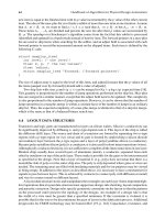
the polygon (see Figure 5.5). We now present an algorithm called Graham’s scan for generating a
convex hull of n points on a plane.
Graham Scan(n points on a plane)
Let p
0
be the point with minimum y coordinate
Sort the rest of the points p
1
, ,p
n−1
by the polar
angle in counterclockwise order w.r.t. p
0
Alpert/Handbook of Algorithms for Physical Design Automation AU7242_C005 Finals Page 86 23-9-2008 #15
86 Handbook of Algorithms for Physical Design Automation
Convex hull
Voronoi diagrams Delaunay triangulation
FIGURE 5.5 Computational geometry.

Initialize Stack S
Push(p
0
,S)
Push(p
1
,S)
Push(p
2
,S)
For i = 3ton−1
While (the angle made by the next to top point on S,
top point on S and p
i
makes a non left turn)
Pop(S)
Push(p
i
,S)
Return S
The algorithm returns the stack S that contains the vertices o f the convex hull. Basically, the
algorithm starts with the bottom-most point p
0
. Then it sorts all the other points in increasing order
of the polar angle made in counterclockwise direction w.r.t p
0
. It then pushes p
0
, p
1

,andp
2
in the
stack. Starting from p
3
, it checks if top two elements and the current point p
i
forms a left turn or not.
If it does then p
i
is pushed into the stack (implying that it is part o f the hull). If not then that means
the current stack has some points not on the convex hull and therefore needs to be popped. Convex
hulls, just like MSTs, are also used in predicting the wirelength when the placement is fixed and
routing is not known.
5.7.2 VORONOI DIAGRAMS AND DELAUNAY TRIANGULATION
A Voronoi diagram is a partitioning of a plane with n points (let us call them central points) into
convex polygons (see Figure 5.5). Each convex polygon has exactly one central point. Also, any
point within the convex polygon is closest to the central point associated with the polygon.
Delaunay triangulation is simply the dual of Voronoi diagrams. This is a triangulation of central
points such that none of the central points are inside the circumcircle of a triangle (see Figure 5.5).
Although we have defined these concepts for a plane, they are easily extendible to multiple
dimensions as well.
5.8 SIMULATED ANNEALING
Simulated annealing is a general global optimization scheme. This technique is primarily inspired
from the process of annealing (slow cooling) in metallurgy where the material is cooled slowly to
form high quality crystals. The simulated annealing algorithm basically follows a similar principle.
Conceptually, it has a startin g temperature parameter that is usually set to a very high quantity. This
Alpert/Handbook of Algorithms for Physical Design Automation AU7242_C005 Finals Page 87 23-9-2008 #16
Basic Algorithmic Techniques 87
temperature p arameter is reduced slowly using a predecided profile. At each temperature value, a

set o f randomly generated moves span the solution space. The moves basically change the current
solution r andomly. A move is accepted if it generates a better solution. If a move generates a solution
quality that is worse than the current one then it can either be accepted or rejected depending on
a random criterion. Essentially, outright rejection of bad solutions may result in the optimization
process getting stuck in local optimum points. Accepting some bad solutions (and remembering th e
best solution found so far) helps us get out of these local optimums and move toward the global
optimum. At a given temperature, a bad solution is accepted if the probability of acceptance is
greater than the randomness associated with the solution. The pseudocode of simulated annealing is
as follows:
Simulated Annealing
s:= Initial Solution s0; c = Cost(s); T = Initial Temperature Tmax
current best solution = s
While (T > Final Temperaure Tmin)
K = 0
While (K <= Kmax)
Accept = 0
s1 = Randomly Perturb Solution(s)
If(cost(s1) < cost(s))
Accept = 1
Else
r = random number between [0,1] with uniform
probability
if (r < exp(−L(cost(s) − cost(s1))/T))
\
∗
Here L is a constant
∗
\
Accept = 1
If Accept = 1

s = s1
If (cost(s1) < cost(current best solution))
current best solution = s1
k = k + 1
T = T
∗
(scaling ´α)
Simulated annelaing has found widespread application in several physical design problems like
placement, floorplanning, etc. [6]. Many successful commerical and academic implementations
of simulated annealing-based gate placement tools have made a large impact on the VLSI CAD
community.
REFERENCES
1. T.H. Cormen, C.L. Leiserson, R.L. Rivest, and C. Stein, Introduction to Algorithms, The MIT Press,
Cambridge, Massachusetts, 2001.
2. G. Chartrand and O.R. Oellermann, Applied and Algorithmic Graph Theory, McGraw-Hill, Singapore,
1993.
3. M.R. Garey and D.S. Johnson, Computers and Intractability: A Guide to the Theory of NP-Completeness,
W.H. Freeman and Company, New York, 1999.
4. R.K. Ahuja, T.L. Magnanti, and J.B. Orlin, Network Flows: Theory, Algorithms and Applications, Prentice
Hall, Englew ood Clif fs, New Jersey, 1993.
5. G. De Micheli, Synthesis and Optimization of Digital Circuits, McGraw-Hill, New York, 1994.
6. M. Sarrafzadeh and C.K. Wong, An Introduction to VLSI Physical Design, McGraw-Hill, New York, 1996.
Alpert/Handbook of Algorithms for Physical Design Automation AU7242_C005 Finals Page 88 23-9-2008 #17
Alpert/Handbook of Algorithms for Physical Design Automation AU7242_C006 Finals Page 89 23-9-2008 #2
6
Optimization Techniques for
Circuit Design Applications
Zhi-Quan Luo
CONTENTS
6.1 Introduction 89

6.2 Optimization Concepts 90
6.2.1 Convex Sets 90
6.2.2 Convex Cones 91
6.2.3 Convex Functions 91
6.2.4 Convex Optimization Problems 92
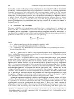
6.3 Lagrangian Duality and the Karush–Kuhn–Tucker Condition 94
6.3.1 Lagrangian Relaxation 96
6.3.2 Detecting Infeasibility 98
6.4 Linear Conic Optimization Models 99
6.4.1 Linear Programming 99
6.4.2 Second-Order Cone Programming 99
6.4.3 Semidefinite Programming 100
6.5 Interior Point Methods for Linear Conic Optimization 100
6.6 Geometric Programming 102
6.6.1 Basic Definitions 102
6.6.2 Convex Reformulation of a GP 102
6.6.3 Gate Sizing as a GP 103
6.7 Robust Optimization 104
6.7.1 Robust Circuit Optimization under Process Variations 105
Acknowledgment 108
References 108
6.1 INTRODUCTION
This chapter describes fundamental concepts and theory o f optimization that are most relevant to
physical design applications. The basic convex optimization models of linear programming (LP),
second-order cone programming, semidefinite programming (SDP), and geometric programming
are reviewed, as are the concept of convexity, optimality conditions, and Lagrangian relaxation.
Finally, the concept of robust optimization is introduced and a circuit optimization example is used
to illustrate its effectiveness.
The goal of this chapter is to provide an overview of these developments and describe the basic
optimization concepts, models, and tools that are most relevant to circuit design applications, and

in particular, to expose the reader to the types of nonlinear optimization problems that are “easy.”
Generally speaking, any problem that can be formulated as a linear program falls into this catego ry.
Thanks to the results of research in the last few years, there are also classes of nonlinear programs
that can now be solved in computationally efficient ways.
89
Alpert/Handbook of Algorithms for Physical Design Automation AU7242_C006 Finals Page 90 23-9-2008 #3
90 Handbook of Algorithms for Physical Design Automation
Until recently, the work-horse algorithms for nonlinear optimization in engineering design have
been the gradient descent method, Newton’s method, and the method of least squares. Although
these algorithms have served their purpose well, they suffer from slow convergence and sensitivity
to the algorithm initialization and stepsize selection, especially when applied to ill-conditioned or
nonconvex problem formulations. This is unfortunate because many design and implementation
problems in circuit design applications naturally lead to nonconvex optimization formulations, the
solution of which by the standard gradient descent or Newton’s algorithm usually works poorly.
The main problem with applying the least squares or the gradient descent algorithms directly to
the nonconvex formulations is slow convergence and local minima. One powerful way to avoid
these problems is to derive an exact convex reformulation of the original nonconvex formulation.
Once a convex reformulation is obtained, we can be guaranteed of finding the globally optimal
design efficiently without the usual headaches of stepsize selection, algorithm initialization, and
local minima. There has been a significant advance in the research of interior point methods [8] and
conic optimization [11] over the last two decades, and the algorithmic framework of interior point
algorithms for solving these convex optimization models are presented.
For some engineering applications, exact linear or convex reformulation is not always possible,
especially when the underlying optimization problem is NP-hard. In such cases, it m ay still be
possible to derive a tight convex relaxation and use the advanced conic optimization techniques to
obtain high-quality approximate solutions for the original NP-hard problem. One general approach
to derive a convex relaxation for an nonconvex optimization problem is via Lagrangian relaxation.
For example, some circuit design applications may involve integer variables that are coupled by
a set of complicating constraints. For these problems, we can bring these coupling constraints to
the objective function in a Lagrangian fashion with fixed multipliers that are changed iteratively.

This Lagrangian relaxation approach removes the complicating constraints from the constraint set,
resulting in considerably easier to solve subproblems. The problem of optimally choosing dual
multipliers is always convex and is ther e fore amenable to efficient solution by the standard convex
optimization techniques.
To recognize convexoptimization problems inengineeringapplications, onemust first be familiar
with the basic concepts of convexity and the commonly used convex optimization models. This
chapter starts with a concise review of these optimization concepts and models including linear
programming,second-order cone programming (SOCP), semidefinite cone programming, as well as
geometric programming, all illustrated through concrete examples. In addition, the Karush–Kuhn–
Tucker optimality conditions are reviewed and stated explicitly for each of the convex optimization
models, followed by a description of the well-known interior point algorithms and a brief discussion
of their worst-case complexity. The chapter concludes with an example illustra ting the use of robust
optimization techniques for a circuit design problem under process variations.
Throughout this chapter, we use lowercase letters to denote vectors, and capital letters to
denote matrices. We use superscript
T
to denote (vector) matrix transpose. Moreover, we denote
the set of n by n symmetric matrices by S
n
, denote the set of n by n positive (semi) definite matrices
(S
n
++
)S
n
+
. For two given matrices X and Y ,weuse“X  Y ”(X  Y) to indicate that X −Y is positive
(semi)-definite, and X •Y:=

i,j

X
ij
Y
ij
= tr XY
T
to indicate the matrix inner product. The Frobenius
norm of X is denoted by X
F
=
√
tr XX
T
. The Euclidean norm of a vector x ∈
n
is denoted x.
6.2 OPTIMIZATION CONCEPTS
6.2.1 C
ONVEX SETS
AsetS ⊂
n
is said to be convex if for any two points x, y ∈ S, the line segment joining x and y also
lies in S. Mathematically, it is defined by the following property
θx + (1 − θ)y ∈ S, ∀ θ ∈[0, 1] and x, y ∈ S.
Alpert/Handbook of Algorithms for Physical Design Automation AU7242_C006 Finals Page 91 23-9-2008 #4
Optimization Techniques for Circuit Design Applications 91
Many well-known sets are convex. For example, the unit ball S ={x |x≤1}. However, the unit
sphere S ={x |x=1} is not convex because the line segment joining any two distinct points is
no longer on the unit sphere. In general, a convex set must be a solid body, containing no holes, and
always curved outward. Other examples of convex sets include ellipsoids, hypercubes, and so on.

In the context of linear programming, the constraining inequalities geometrically form a polyhedral
set, which is easily shown to be convex.
In the real line , convex sets correspond to intervals (open or closed). The most important
property about convex set is the fact that the intersection of any number (possibly uncountable) of
convex sets remains convex. For example, the set S ={x |x≤1, x ≥ 0} is the intersection of the
unit ball with the nonnegative orthant (
n
+
), both of which are convex. Thus, their intersection S is
also convex. The unions of two convex sets are typically nonconvex.
6.2.2 CONVEX CONES
A convex cone K is a special type of convex set that is closed under positive scaling: for each x ∈ K
and each α ≥ 0, αx ∈ K. Convex cones arise in various forms in engineering applications. The most
common convex cones are
1. Nonnegative orthant 
n
+
2. Second-order cone (also known as ice-cream cone):
K = SOC(n) ={(t, x) | t ≥x}
3. Positive semidefinite matrix cone
K = S
n
+
={X | X symmetric and X  0}
For any convex cone K, we can define its dual cone
K
∗
={x |x, y≥0, ∀ y ∈ K}
where ·, · denotes the inner product operation. In other words, the dual cone K
∗

consists of all
vectors y that form a nonobtuse angle with all vectors in K. We will say K is self-dual if K = K
∗
.It
can be shown that the nonnegative orthant cone, the second-order cone, and the symmetric positive
semidefinite matrix cone are all self-dual. Notice that for the second-order cone, the inner product
operation ·, · is defined as
(t, x), (s, y)=ts + x
T
y,forall(t, x) and (s, y) with t ≥x and s ≥y
and for the positive semidefinite m atrix cone
X, Y =X • Y =

i,j
X
ij
Y
ij
6.2.3 CONVEX FUNCTIONS
A function f (x): 
n
→is said to be convex if for any two points x, y ∈
n
f (θ x +(1 − θ)y) ≤ θ f (x) +(1 −θ)f (y), ∀θ ∈[0, 1]
Geometrically, this means that, when restricted over the line segment joining x and y, the linear
function joining (x, f (x)) and (y, f (y)) always dominates the function f .