7.5 Cholesky Factorization for Sparse Matrices 433
express the specific situation of data dependences between columns using the rela-
tion parent( j) [124, 118]. For each column j,0≤ j < n, we define
parent ( j) = min{i |i ∈ Struct(L
∗j
)} if Struct(L
∗j
) =∅,
i.e., parent (j) is the row index of the first off-diagonal non-zero of column j.If
Struct(L
∗j
) =∅, then parent(j) = j. The element parent ( j) is the first column
i > j which depends on j. A column l, j < l < i, between them does not depend
on j, since j /∈ Struct(L
l∗
) and no cmod(l, j) is executed. Moreover we define for
0 ≤ i < n
children(i) ={j < i |parent ( j) = i},
i.e., children(i) contains all columns j that have their first off-diagonal non-zero in
row i.
The directed graph G = (V, E) has a set of nodes V ={0, ,n −1} with one
node for each column and a set of edges E, where (i, j) ∈ E if i = parent( j) and
i = j. It can be shown that G isatreeifmatrixA is irreducible.(AmatrixA is
called reducible if A can be permuted such that it is block-diagonal. For a reducible
matrix, the blocks can be factorized independently.) In the following, we assume
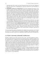
an irreducible matrix. Figure 7.25 shows a matrix and its corresponding elimination
tree.
In the following, we denote the subtree with root j by G[ j]. For sparse Cholesky
factorization, an important property of the elimination tree G is that the tree spec-
ifies the order in which the columns must be evaluated: The definition of parent
implies that column i must

be evaluated before column j,ifj = parent (i). Thus,
all the children of column j must be completely evaluated before the computation
of j. Moreover, column j does not depend on any column that is not in the subtree
G[ j]. Hence, columns i and j can be computed in parallel, if G[i] and G[j]are
disjoint subtrees. Especially, all leaves of the elimination tree can be computed in
parallel and the computation does not need to start with column 0. Thus, the sparsity
structure determines the parallelism to be exploited. For a given matrix, elimination
trees of smaller height usually represent a larger degree of parallelism than trees of
larger height [77].
0
1
2
3
4
5
6
7
8
9
∗
∗
∗
∗
∗∗
∗
∗∗
∗
∗∗∗∗∗
∗∗∗∗∗∗∗∗∗∗
0123456789

9
02578
6 3
4
1
Fig. 7.25 Sparse matrix and the corresponding elimination tree
434 7 Algorithms for Systems of Linear Equations
7.5.3.1 Parallel Left-Looking Algorithms
The parallel implementation of the left-looking algorithm (III) is based on n col-
umn tasks Tcol(0), ,Tcol(n −1) where task Tcol( j), 0 ≤ j < n, comprises the
execution of cmod( j, k) for all k ∈ Struct(L
j∗
) and the execution of cdiv( j); this
is the loop body of the for loop in algorithm (III). These tasks are not indepen-
dent of each other but have dependences due to the non-zero elements. The parallel
implementation uses a task pool for managing the execution of the tasks. The task
pool has a central task pool for storing column tasks, which can be accessed by
every processor. Each processor is responsible for performing a subset of the column
tasks. The assignment of tasks to processors for execution is dynamic, i.e., when a
processor is idle, it takes a task from the central task pool.
The dynamic implementation has the advantage that the workload is distributed
evenly although the tasks might have different execution times due to the sparsity
structure. The concurrent accesses of the processors to the central task pool have to
be conflict-free so that the unique assignment of a task to a processor for execution
is guaranteed. This can be implemented by a locking mechanism so that only one
processor accesses the task pool at a specific time.
There are several parallel implementation variants for the left-looking algorithm
differing in the way the column tasks are inserted into the task pool. We consider
three implementation variants:
• Variant L1 inserts column task Tcol( j) into the task pool not before all column

tasks Tcol(k) with k ∈ Struct(L
j∗
) have been finished. The task pool can be ini-
tialized to the leaves of the elimination tree. The degree of parallelism is limited
by the number of independent nodes of the tree, since tasks dependent on each
other are executed in sequential order. Hence, a processor that has accessed task
Tcol( j) can execute the task without waiting for other tasks to be finished.
• Variant L2 allows to start the execution of Tcol( j) without requiring that it can
be executed to completion immediately. The task pool is initialized to all column
tasks available. The column tasks are accessed by the processors dynamically
from left to right, i.e., an idle processor accesses the next column that has not yet
been assigned to a processor.
The computation of column task Tcol( j) is started before all tasks Tcol(k)
with k ∈ Struct(L
j∗
) have been finished. In this case, not all operations
cmod( j, k)ofTcol( j) can be executed immediately but the task can perform
only those cmod( j, k) operations with k ∈ Struct(L
j∗
) for which the corre-
sponding tasks have already been executed. Thus, the task might have to wait
during its execution for other tasks to be finished.
To control the execution of a single column task Tcol ( j), each column j is
assigned a data structure S
j
containing all columns k ∈ Struct(L
j∗
)forwhich
cmod( j, k) can already be executed. When a processor finishes the execution
of the column task Tcol(k) (by executing cdiv(k)), it pushes k onto the data

structures S
j
for each j ∈ Struct(L
∗k
). Because different processors might try
to access the same stack at the same time, a locking mechanism has to be used
to avoid access conflicts. The processor executing Tcol( j) pops column indices
7.5 Cholesky Factorization for Sparse Matrices 435
Fig. 7.26 Parallel
left-looking algorithm
according to variant L2. The
implicit task pool is
implemented in the while
loop and the function
get
unique index().
The stacks S
1
, ,S
n
implement the bookkeeping
about the dependent columns
already finished
k from S
j
and executes the corresponding cmod( j, k) operation. If S
j
is empty,
the processor waits for another processor to insert new column indices. When
|Struct(L

j∗
)| column indices have been retrieved from S
j
,thetaskTcol( j) can
execute the final cdiv( j) operation.
Figure 7.26 shows the corresponding implementation. The central task pool
is realized implicitly as a parallel loop; the operation get
unique index()
ensures a conflict-free assignment of tasks so that the processors accessing the
pool at the same time get different unique loop indices representing column tasks.
The loop body of the while loop implements one task Tcol( j). The data struc-
tures S
1
, ,S
n
are stacks; pop(S
j
) retrieves an element and push( j, S
i
) inserts
an element onto the stack.
• Variant L3 is a variation of L2 that takes the structure of the elimination tree into
consideration. The columns are not assigned strictly from left to right to the pro-
cessors, but according to their height in the elimination tree, i.e., the children of a
column j in the elimination tree are assigned to processors before their parent j.
This variant tries to complete the column tasks in the order in which the columns
are needed for the completion of the other columns, thus exploiting the additional
parallelism that is provided by the sparsity structure of the matrix.
7.5.3.2 Parallel Right-Looking Algorithm
The parallel implementation of the right-looking algorithm (IV) is also based on a

task pool and on column tasks. These column tasks are defined differently than the
tasks of the parallel left-looking algorithm: A column task Tcol( j), 0 ≤ j < n,
comprises the execution of cdiv( j) and cmod(k, j) for all k ∈ Struct(L
∗j
), i.e., a
column task comprises the final computation for column j and the modifications of
all columns k > j right of column j that depend on j. The task pool is initialized to
all column tasks corresponding to the leaves of the elimination tree. A task Tcol( j)
that is not a leaf is inserted into the task pool as soon as the operations cmod( j, k)
for all k ∈ Struct(L
j∗
) are executed and a final cdiv( j) operation is possible.
Figure 7.27 sketches a parallel implementation of the right-looking algorithm.
The task assignment is implemented by maintaining a counter c
j
for each col-
umn j. The counter is initialized to 0 and is incremented after the execution of
each cmod( j, ∗) operation by the corresponding processor using the conflict-free
436 7 Algorithms for Systems of Linear Equations
Fig. 7.27 Parallel right-looking algorithm. The column tasks are managed by a task pool TP.
Column tasks are inserted into the task pool by add
column() and retrieved from the task
pool by get
column(). The function initialize task pool() initializes the task pool
TP with the leaves of the elimination tree. The condition of the outer while loop assigns column
indices j to processors. The processor retrieves the corresponding column task as soon as the call
filled
pool(TP,j) returns that the column task exists in the task pool
procedure add counter(). For the execution of a cmod(k, j) operation of a task
Tcol( j), column k must be locked to prevent other tasks from modifying the same

column at the same time. A task Tcol( j) is inserted into the task pool, when the
counter c
j
has reached the value |Struct(L
j∗
)|.
The differences between this right-looking implementation and the left-looking
variant L2 lie in the execution order of the cmod() operations and in the executing
processor. In the L2 variant, the operation cmod( j, k) is initiated by the processor
computing column k by pushing it on stack S
j
, but the operation is executed by
the processor computing column j. This execution need not be performed immedi-
ately after the initiation of the operation. In the right-looking variant, the operation
cmod( j, k) is not only initiated, but also executed by the processor that computes
column k.
7.5.3.3 Parallel Supernodal Algorithm
The parallel implementation of the supernodal algorithm uses a partition into funda-
mental supernodes. A supernode I(p) ={p, p +1, , p +q −1} is a fundamental
supernode, if for each i with 0 ≤ i ≤ q −2, we have children(p +i +1) ={p +i},
i.e., node p + i is the only child of p + i + 1 in the elimination tree [124]. In
Fig. 7.23, supernode I (2) ={2, 3, 4} is a fundamental supernode whereas supern-
odes I (6) ={6, 7} and I (8) ={8, 9} are not fundamental. In a partition into fun-
damental supernodes, all columns of a supernode can be computed as soon as the
first column can be computed and a waiting for the computation of columns outside
the supernode is not needed. In the following, we assume that all supernodes are
fundamental, which can be achieved by splitting supernodes into smaller ones. A
supernode consisting of a single column is fundamental.
The parallel implementation of the supernodal algorithm (VI)
is based on

supernode tasks Tsup(J) where task Tsup(J)for0≤ J < N comprises the
7.6 Exercises for Chap. 7 437
execution of smod( j, J) and cdiv( j) for each j ∈ J from left to right and the
execution of smod(k, J) for all k ∈ Struct(L
∗(last(J))
); N is the number of supern-
odes. Tasks Tsup(J ) that are ready for execution are held in a central task pool that
is accessed by the idle processors. The pool is initialized to supernodes that are ready
for completion; these are those supernodes whose first column is a leaf in the elim-
ination tree. If the execution of a cmod(k, J ) operation by a task Tsup(J) finishes
the modification of another supernode K > J, the corresponding task Tsup(K)is
inserted into the task pool.
The assignment of supernode tasks is again implemented by maintaining a
counter c
j
for each column j of a supernode. Each counter is initialized to 0 and
is incremented for each modification that is executed for column j. Ignoring the
modifications with columns inside a supernode, a supernode task Tsup(J) is ready
for execution if the counters of the columns j ∈ J reach the value |Struct(L
j∗
)|.
The implementation of the counters as well as the manipulation of the columns has
to be protected, e.g., by a lock mechanism. For the manipulation of a column k /∈ J
by a smod(k, J) operation, column k is locked to avoid concurrent manipulation by
different processors. Figure 7.28 shows the corresponding implementation.
Fig. 7.28 Parallel supernodal
algorithm
7.6 Exercises for Chap. 7
Exercise 7.1 For an n ×m matrix A and vectors a and b of length n write a parallel
MPI program which computes a rank-1 update A = A − a · b

T
which can be
computed sequentially by
for (i=0; i<n; i++)
for (j=0; j<n; j++)
A[i][j] = A[i][j]-a[i] · b[j];
438 7 Algorithms for Systems of Linear Equations
For the parallel MPI implementation assume that A is distributed among the p pro-
cessors in a column-cyclic way. The vectors a and b are available at the process
with rank 0 only and must be distributed appropriately before the computation.
After the update operation, the matrix A should again be distributed in a column-
cyclic way.
Exercise 7.2 Implement the rank-1 update in OpenMP. Use a parallel for loop to
express the parallel execution.
Exercise 7.3 Extend the program piece in Fig. 7.2 for performing the Gaussian
elimination with a row-cyclic data distribution to a full MPI program. To do so,
all helper functions used and described in the text must be implemented. Measure
the resulting execution times for different matrix sizes and different numbers of
processors.
Exercise 7.4 Similar to the previous exercise, transform the program piece in Fig. 7.6
with a total cyclic data distribution to a full MPI program. Compare the resulting
execution times for different matrix sizes and different numbers of processors. For
which scenarios does a significant difference occur? Try to explain the observed
behavior.
Exercise 7.5 Develop a parallel implementation of Gaussian elimination for shared
address spaces using OpenMP. The MPI implementation from Fig. 7.2 can be
used as an orientation. Explain how the available parallelism is expressed in your
OpenMP implementation. Also explain where synchronization is needed when
accessing shared data. Measure the resulting execution times for different matrix
sizes and different numbers of processors.

Exercise 7.6 Develop a parallel implementation of Gaussian elimination using Java
threads. Define a new class Gaussian which is structured similar to the Java
program in Fig. 6.23 for a matrix multiplication. Explain which synchronization
is needed in the program. Measure the resulting execution times for different matrix
sizes and different numbers of processors.
Exercise 7.7 Develop a parallel MPI program for Gaussian elimination using a
column-cyclic data distribution. An implementation with a row-cyclic distribution
has been given in Fig. 7.2. Explain which communication is needed for a column-
cyclic distribution and include this communication in your program. Compute
the resulting speedup values for different matrix sizes and different numbers of
processors.
Exercise 7.8 For n = 8 consider the following tridiagonal equation system:
⎛
⎜
⎜
⎜
⎜
⎜
⎜
⎝
11
12 1
12
.
.
.
.
.
.
.

.
.
1
12
⎞
⎟
⎟
⎟
⎟
⎟
⎟
⎠
· x =
⎛
⎜
⎜
⎜
⎜
⎜
⎝
1
2
3
.
.
.
8
⎞
⎟
⎟

⎟
⎟
⎟
⎠
.
7.6 Exercises for Chap. 7 439
Use the recursive doubling technique from Sect. 7.2.2, p. 385, to solve this equation
system.
Exercise 7.9 Develop a sequential implementation of the cyclic reduction algorithm
for solving tridiagonal equation systems, see Sect. 7.2.2, p. 385. Measure the result-
ing sequential execution times for different matrix sizes starting with size n = 100
up to size n = 10
7
.
Exercise 7.10 Transform the sequential implementation of the cyclic reduction
algorithm from the last exercise into a parallel implementation for a shared address
space using OpenMP. Use an appropriate parallel for loop to express the paral-
lel execution. Measure the resulting parallel execution times for different numbers
of processors for the same matrix sizes as in the previous exercise. Compute the
resulting speedup values and show the speedup values in a diagram.
Exercise 7.11 Develop a parallel MPI implementation of the cyclic reduction algo-
rithm for a distributed address space based on the description in Sect. 7.2.2, p. 385.
Measure the resulting parallel execution times for different numbers of processors
and compute the resulting speedup values.
Exercise 7.12 Specify the data dependence graph for the cyclic reduction algorithm
for n = 12 equations according to Fig. 7.11. For p = 3 processors, illustrate the
three phases according to Fig. 7.12 and show which dependences lead to communi-
cation.
Exercise 7.13 Implement a parallel Jacobi iteration with a pointer-based storage
scheme of the matrix A such that global indices are used in the implementation.

Exercise 7.14 Consider the parallel implementation of the Jacobi iteration in
Fig. 7.13 and provide a corresponding shared memory program using OpenMP
operations.
Exercise 7.15 Implement a parallel SOR method for a dense linear equation system
by modifying the parallel program in Fig. 7.14.
Exercise 7.16 Provide a shared memory implementation of the Gauss–Seidel method
for the discretized Poisson equation.
Exercise 7.17 Develop a shared memory implementation for Cholesky factorization
A = LL
T
for a dense matrix A using the basic algorithm.
Exercise 7.18 Develop a message-passing implementation for dense Cholesky fac-
torization A = LL
T
.
440 7 Algorithms for Systems of Linear Equations
Exercise 7.19 Consider a matrix with the following non-zero entries:
0123456789
0
1
2
3
4
5
6
7
8
9
⎛
⎜

⎜
⎜
⎜
⎜
⎜
⎜
⎜
⎜
⎜
⎜
⎜
⎜
⎜
⎝
∗
∗∗
∗
∗∗
∗∗∗
∗∗∗∗∗∗
∗
∗∗∗ ∗
∗∗ ∗ ∗∗
∗∗∗∗∗ ∗∗
⎞
⎟
⎟
⎟
⎟
⎟

⎟
⎟
⎟
⎟
⎟
⎟
⎟
⎟
⎟
⎠
(a) Specify all supernodes of this matrix.
(b) Consider a supernode J with at least three entries. Specify the sequence of
cmod and cdiv operations that are executed for this supernode in the right-looking
supernode Cholesky factorization algorithm.
(c) Determine the elimination tree resulting for this matrix.
(d) Explain the role of the elimination tree for a parallel execution.
Exercise 7.20 Derive the parallel execution time of a message-passing program of
the CG method for a distributed memory machine with a linear array as intercon-
nection network.
Exercise 7.21 Consider a parallel implementation of the CG method in which the
computation step (3) is executed in parallel to the computation step (4). Given a row-
blockwise distribution of matrix A and a blockwise distribution of the vector, derive
the data distributions for this implementation variant and give the corresponding
parallel execution time.
Exercise 7.22 Implement the CG algorithm given in Fig. 7.20 with the blockwise
distribution as message-passing program using MPI.
References
1. F. Abolhassan, J. Keller, and W.J. Paul. On the Cost–Effectiveness of PRAMs. In Proceedings
of the 3rd IEEE Symposium on Parallel and Distributed Processing, pages 2–9, 1991.
2. A. Adl-Tabatabai, C. Kozyrakis, and B. Saha. Unlocking concurrency. ACM Queue, 4(10):

24–33, Dec 2006.
3. S.V. Adve and K. Gharachorloo. Shared memory consistency models: A tutorial. IEEE
Computer, 29: 66–76, 1995.
4. A. Aggarwal, A.K. Chandra, and M. Snir. On Communication Latency in PRAM Compu-
tations. In Proceedings of 1989 ACM Symposium on Parallel Algorithms and Architectures
(SPAA’89), pages 11–21, 1989.
5. A. Aggarwal, A.K. Chandra, and M. Snir. Communication complexity of PRAMs. Theoreti-
cal Computer Science, 71: 3–28, 1990.
6. A. Aho, M. Lam, R. Sethi, and J. Ullman. Compilers: Principles, Techniques & Tools.
Pearson-Addison Wesley, Boston, 2007.
7. A.V. Aho, M.S. Lam, R. Sethi, and J.D. Ullman. Compilers: Principles, Techniques, and
Tools. 2nd Edition, Addison-Wesley Longman Publishing Co., Inc., Boston, 2006.
8. S.G. Akl. Parallel Computation – Models and Methods. Prentice Hall, Upper Saddle River,
1997.
9. K. Al-Tawil and C.A. Moritz. LogGP Performance Evaluation of MPI. International Sympo-
sium on High-Performance Distributed Computing, page 366, 1998.
10. A. Alexandrov, M. Ionescu, K.E. Schauser, and C. Scheiman. LogGP: Incorporating Long
Messages into the LogP Model – One Step Closer Towards a Realistic Model for Parallel
Computation. In Proceedings of the 7th ACM Symposium on Parallel Algorithms and Archi-
tectures (SPAA’95), pages 95–105, Santa Barbara, July 1995.
11. E. Allen, D. Chase, J. Hallett, V. Luchangco, J W. Maessen, S. Ryu, G.L. Steele, Jr., and
S. Tobin-Hochstadt. The Fortress Language Specification, version 1.0 beta, March 2007.
12. R. Allen and K. Kennedy. Optimizing Compilers for Modern Architectures. Morgan
Kaufmann, San Francisco, 2002.
13. S. Allmann, T. Rauber, and G. R
¨
unger. Cyclic Reduction on Distributed Shared Memory
Machines. In Proceedings of the 9th Euromicro Workshop on Parallel and Distributed Pro-
cessing, pages 290–297, Mantova, Italien, 2001. IEEE Computer Society Press.
14. G.S. Almasi and A. Gottlieb. Highly Parallel Computing. Benjamin Cummings, New York,

1994.
15. G. Amdahl. Validity of the Single Processor Approach to Achieving Large-Scale Computer
Capabilities. In AFIPS Conference Proceedings, volume 30, pages 483–485, 1967.
16. K. Asanovic, R. Bodik, B.C. Catanzaro, J.J. Gebis, P. Husbands, K. Keutzer, D.A. Patterson,
W.L. Plishker, J. Shalf, S.W. Williams, and K.A. Yelick. The Landscape of Parallel Com-
puting Research: A View from Berkeley. Technical Report UCB/EECS-2006–183, EECS
Department, University of California, Berkeley, December 2006.
T. Rauber, G. R
¨
unger, Parallel Programming,
DOI 10.1007/978-3-642-04818-0,
C

Springer-Verlag Berlin Heidelberg 2010
441
442 References
17. M. Azimi, N. Cherukuri, D.N. Jayasimha, A. Kumar, P. Kundu, S. Park, I. Schoinas, and
A. Vaidya. Integration challenges and tradeoffs for tera-scale architectures. Intel Technology
Journal, 11(03), 2007.
18. C.J. Beckmann and C. Polychronopoulos. Microarchitecture Support for Dynamic Schedul-
ing of Acyclic Task Graphs. Technical Report CSRD 1207, University of Illinois, 1992.
19. D.P. Bertsekas and J.N. Tsitsiklis. Parallel and Distributed Computation. Athena Scientific,
Nashua, 1997.
20. R. Bird. Introduction to Functional Programming Using Haskell. Prentice Hall, Englewood
Cliffs, 1998.
21. P. Bishop and N. Warren. JavaSpaces in Practice. Addison Wesley, Reading, 2002.
22. F. Bodin, P. Beckmann, D.B. Gannon, S. Narayana, and S. Yang. Distributed C++:Basic
Ideas for an Object Parallel Language. In Proceedings of the Supercomputing’91 Conference,
pages 273–282, 1991.
23. D. Braess. Finite Elements. 3rd edition, Cambridge University Press, Cambridge, 2007.

24. P. Brucker. Scheduling Algorithms. 4th edition, Springer-Verlag, Berlin, 2004.
25. D.R. Butenhof. Programming with POSIX Threads. Addison-Wesley Longman Publishing
Co., Inc., Boston, 1997.
26. N. Carriero and D. Gelernter. Linda in Context. Communications of the ACM, 32(4):
444–458, 1989.
27. N. Carriero and D. Gelernter. How to Write Parallel Programs. MIT Press, Cambridge,
1990.
28. P. Charles, C. Grothoff, V.A. Saraswat, C. Donawa, A. Kielstra, K. Ebcioglu, C. von Praun,
and V. Sarkar. X10: An Object-Oriented Approach to Non-uniform Cluster Computing. In
R. Johnson and R.P. Gabriel, editors, Proceedings of the 20th Annual ACMSIGPLAN Confer-
ence on Object-Oriented Programming, Systems, Languages, and Applications (OOPSLA),
pages 519–538, ACM, October 2005.
29. A. Chin. Complexity Models for All-Purpose Parallel Computation. In Lectures on Parallel
Computation, chapter 14. Cambridge University Press, Cambridge, 1993.
30. M.E. Conway. A Multiprocessor System Design. In Proceedings of the AFIPS 1963 Fall
Joint Computer Conference, volume 24, pages 139–146, Spartan Books, New York, 963.
31. T.H. Cormen, C.E. Leiserson, and R.L. Rivest. Introduction to Algorithms. MIT Press,
Cambridge, 2001.
32. D.E. Culler, A.C. Arpaci-Dusseau, S.C. Goldstein, A. Krishnamurthy, S. Lumetta, T. van
Eicken, and K.A. Yelick. Parallel Programming in Split-C. In Proceedings of Supercomput-
ing, pages 262–273, 1993.
33. D.E. Culler, A.C. Dusseau, R.P. Martin, and K.E. Schauser. Fast Parallel Sorting Under
LogP: From Theory to Practice. In Portability and Performance for Parallel Processing,
pages 71–98. Wiley, Southampton, 1994.
34. D.E. Culler, R. Karp, A. Sahay, K.E. Schauser, E. Santos, R. Subramonian, and T. von Eicken.
LogP: Towards a Realistic Model of Parallel Computation. Proceedings of the 4th ACM SIG-
PLAN Symposium on Principles and Practice of Parallel Programming (PPoPP’93), pages
1–12, 1993.
35. D.E. Culler, J.P. Singh, and A. Gupta. Parallel Computer Architecture: A Hardware Software
Approach. Morgan Kaufmann, San Francisco, 1999.

36. H.J. Curnov and B.A. Wichmann. A Synthetic Benchmark. The Computer Journal, 19(1):
43–49, 1976.
37. D. Callahan, B.L. Chamberlain, and H.P. Zima. The Cascade High Productivity Language.
In IPDPS, pages 52–60. IEEE Computer Society, 2004.
38. W.J. Dally and C.L. Seitz. Deadlock-Free Message Routing in Multiprocessor Interconnec-
tion Networks. IEEE Transactions on Computers, 36(5): 547–553, 1987.
39. DEC. The Whetstone Performance. Technical Report, Digital Equipment Corporation, 1986.
40. E.W. Dijkstra. Cooperating Sequential Processes. In F. Genuys, editor, Programming Lan-
guages,
pages 43–112. Academic Press Inc., 1968.