7.3 Iterative Methods for Linear Systems 403
x
(k+1)
i
=
ω
a
ii
⎛
⎝
b
i
−
n

j=1, j=i
a
ij
x
(k)
j
⎞
⎠
+(1 −ω)x
(k)
i
, i = 1, ,n . (7.39)
More popular is the modification with a relaxation parameter for the Gauss–Seidel
method, the SOR method.
7.3.1.5 SOR Method
The SOR method or (successive over-relaxation) is a modification of the Gauss–

Seidel iteration that speeds up the convergence of the Gauss–Seidel method by intro-
ducing a relaxation parameter ω ∈ R. This parameter is used to modify the way in
which the combination of the previous approximation x
(k)
and the components of the
current approximation x
(k+1)
1
, ,x
(k+1)
i−1
are combined in the computation of x
(k+1)
i
.
The (k + 1)th approximation computed according to the Gauss–Seidel iteration
(7.38) is now considered as intermediate result
ˆ
x
(k+1)
and the next approximation
x
(k+1)
of the SOR method is computed from both vectors
ˆ
x
(k+1)
and x
(k+1)
in the

following way:
ˆ
x
(k+1)
i
=
1
a
ii
⎛
⎝
b
i
−
i−1

j=1
a
ij
x
(k+1)
j
−
n

j=i+1
a
ij
x
(k)

j
⎞
⎠
, i = 1, ,n , (7.40)
x
(k+1)
i
= x
(k)
i
+ω(
ˆ
x
(k+1)
i
− x
(k)
i
) , i = 1, ,n . (7.41)
Substituting Eq. (7.40) into Eq. (7.41) results in the iteration
x
(k+1)
i
=
ω
a
ii
⎛
⎝
b

i
−
i−1

j=1
a
ij
x
(k+1)
j
−
n

j=i+1
a
ij
x
(k)
j
⎞
⎠
+(1 −ω)x
(k)
i
(7.42)
for i = 1, ,n. The corresponding splitting of the matrix A is A =
1
ω
D − L −
R −

1−ω
ω
D and an iteration step in matrix form is
(D − wL)x
(k+1)
= (1 −ω)Dx
(k)
+ωRx
(k)
+ωb .
The convergence of the SOR method depends on the properties of A and the value
chosen for the relaxation parameter ω. For example the following property holds: If
A is symmetric and positive definite and ω ∈ (0, 2), then the SOR method converges
for every start vector x
(0)
. For more numerical properties see books on numerical
linear algebra, e.g., [23, 61, 71, 166].
7.3.1.6 Implementation Using Matrix Operations
The iteration (7.36) computing x
(k+1)
for a given vector x
(k)
consists of
404 7 Algorithms for Systems of Linear Equations
• a matrix–vector multiplication of the iteration matrix C with x
(k)
and
• a vector–vector addition of the result of the multiplication with vector d.
The specific structure of the iteration matrix, i.e., C
Ja

for the Jacobi iteration
and C
Ga
for the Gauss–Seidel iteration, is exploited. For the Jacobi iteration with
C
Ja
= D
−1
(L + R) this results in the following computation steps:
• a matrix–vector multiplication of L + R with x
(k)
,
• a vector–vector addition of the result with b, and
• a matrix–vector multiplication with D
−1
(where D is a diagonal matrix and thus
D
−1
is easy to compute).
A sequential implementation uses Formula (7.37), and the components x
(k+1)
i
,
i = 1, ,n, are computed one after another. The entire vector x
(k)
is needed
for this computation. For the Gauss–Seidel iteration with C
Ga
= (D − L)
−1

R the
computation steps are
• a matrix–vector multiplication Rx
(k)
with upper triangular matrix R,
• a vector–vector addition of the result with b, and
• the solution of a linear system with lower triangular matrix (D − L).
A sequential implementation uses Formula (7.38). Since the most recently com-
puted approximation components are always used for computing a value x
(k+1)
i
,
the previous value x
(k)
i
can be overwritten. The iteration method stops when the
current approximation is close enough to the exact solution. Since this solution is
unknown, the relative error is used for error control and after each iteration step the
convergence is tested according to
x
(k+1)
− x
(k)
≤εx
(k+1)
, (7.43)
where ε is a predefined error value and . is a vector norm such as x
∞
=
max

i=1, ,n
|x|
i
or x
2
= (

n
i=1
|x
i
|
2
)
1
2
.
7.3.2 Parallel Implementation of the Jacobi Iteration
In the Jacobi iteration (7.37), the computations of the components x
(k+1)
i
, i =
1, ,n, of approximation x
(k+1)
are independent of each other and can be exe-
cuted in parallel. Thus, each iteration step has a maximum degree of potential par-
allelism of n and p = n processors can be employed. For a parallel system with
distributed memory, the values x
(k+1)
i

are stored in the individual local memories.
Since the computation of one of the components of the next approximation requires
all components of the previous approximation, communication has to be performed
to create a replicated distribution of x
(k)
. This can be done by a multi-broadcast
operation.
When considering the Jacobi iteration built up of matrix and vector opera-
tions, a parallel implementation can use the parallel implementations introduced
7.3 Iterative Methods for Linear Systems 405
in Sect. 3.6. The iteration matrix C
Ja
is not built up explicitly but matrix A is
used without its diagonal elements. The parallel computation of the components
of x
(k+1)
corresponds to the parallel implementation of the matrix–vector product
using the parallelization with scalar products, see Sect. 3.6. The vector addition
can be done after the multi-broadcast operation by each of the processors or before
the multi-broadcast operation in a distributed way. When using the parallelization
of the linear combination from Sect. 3.6, the vector addition takes place after the
accumulation operation. The final broadcast operation is required to provide x
(k+1)
to all processors also in this case.
Figure 7.13 shows a parallel implementation of the Jacobi iteration using C nota-
tion and MPI operations from [135]. For simplicity it is assumed that the matrix
size n is a multiple of the number of processors p. The iteration matrix is stored in a
row-blockwise way so that each processor owns n/ p consecutive rows of matrix A
which are stored locally in array local
A. The vector b is stored in a corresponding

blockwise way. This means that the processor me,0≤ me < p,storestherows
me ·n/p +1, ,(me +1) ·n/ p of A in local
A and the corresponding compo-
nents of b in local
b. The iteration uses two local arrays x old and x new for
storing the previous and the current approximation vectors. The symbolic constant
GLOB
MAX is the maximum size of the linear equation system to be solved. The
result of the local matrix–vector multiplication is stored in local
x; local x is
computed according to Eq. (7.37). An MPI
Allgather() operation combines
the local results so that each processor stores the entire vector x
new. The iteration
stops when a predefined number max
it of iteration steps has been performed or
when the difference between x
old and x new is smaller than a predefined value
tol. The function distance() implements a maximum norm and the function
output(x
new,global x) returns array global x which contains the last
approximation vector to be the final result.
7.3.3 Parallel Implementation of the Gauss–Seidel Iteration
The Gauss–Seidel iteration (7.38) exhibits data dependences, since the computation
of the component x
(k+1)
i
, i ∈{1, ,n}, uses the components x
(k+1)
1

, ,x
(k+1)
i−1
of
the same approximation and the components of x
(k+1)
have to be computed one
after another. Since for each i ∈{1, ,n} the computation (7.38) corresponds to a
scalar product of the vector
(x
(k+1)
1
, ,x
(k+1)
i−1
, 0, x
(k)
i+1
, ,x
(k)
n
)
and the ith row of A, this means that the scalar products have to be computed one
after another. Thus, parallelism is only possible within the computation of each sin-
gle scalar product: Each processor can compute a part of the scalar product, i.e., a
local scalar product, and the results are then accumulated. For such an implemen-
tation a column-blockwise distribution of matrix A is suitable. Again, we assume
that n is a multiple of the number p of processors. The approximation vectors are
406 7 Algorithms for Systems of Linear Equations
Fig. 7.13 Program fragment in C notation and with MPI communication operations for a par-

allel implementation of the Jacobi iteration. The arrays local
x, local b,andlocal A are
declared globally. The dimension of local
A is n local ×n. A pointer-oriented storage scheme
as shown in Fig. 7.3 is not used here so that the array indices in this implementation differ from the
indices in a sequential implementation. The computation of local
x[i local] is performed
in two loops with loop index j; the first loop corresponds to the multiplication with array elements
in row i
local to the left of the main diagonal of A and the second loop corresponds to the mul-
tiplication with array elements in row i
local to the right of the main diagonal of A.Theresult
is divided by local
A[i local][i global] which corresponds to the diagonal element of
that row in the global matrix A
7.3 Iterative Methods for Linear Systems 407
distributed correspondingly in a blockwise way. Processor P
q
,1≤ q ≤ p, com-
putes that part of the scalar product for which it owns the columns of A and the
components of the approximation vector x
(k)
. This is the computation
s
qi
=
q·n/p

j=(q−1)·n/ p+1
j<i

a
ij
x
(k+1)
j
+
q·n/p

j=(q−1)·n/ p+1
j>i
a
ij
x
(k)
j
. (7.44)
The intermediate results s
qi
computed by processors P
q
, q = 1, ,p, are accumu-
lated by a single-accumulation operation with the addition as reduction operation
and the value x
(k+1)
i
is the result. Since the next approximation vector x
(k+1)
is
expected in a blockwise distribution, the value x
(k+1)

i
is accumulated at the pro-
cessor owning the ith component, i.e., x
(k+1)
i
is accumulated by processor P
q
with
q =i/(n/ p). A parallel implementation of the SOR method corresponds to the
parallel implementation of the Gauss–Seidel iteration, since both methods differ
only in the additional relaxation parameter of the SOR method.
Figure 7.14 shows a program fragment using C notation and MPI operations of a
parallel Gauss–Seidel iteration. Since only the most recently computed components
of an approximation vector are used in further computations, the component x
(k)
i
is
overwritten by x
(k+1)
i
immediately after its computation. Therefore, only one array
x is needed in the program. Again, an array local
A stores the local part of matrix
A which is a block of columns in this case; n
local is the size of the block. The
for loop with loop index i computes the scalar products sequentially; within the
loop body the parallel computation of the inner product is performed according to
Formula (7.44). An MPI reduction operation computes the components at differing
processors root which finalizes the computation.
7.3.4 Gauss–Seidel Iteration for Sparse Systems

The potential parallelism for the Gauss–Seidel iteration or the SOR method is lim-
ited because of data dependences so that a parallel implementation is only reason-
able for very large equation systems. Each data dependency in Formula (7.38) is
caused by a coefficient (a
ij
)ofmatrixA, since the computation of x
(k+1)
i
depends on
the value x
(k+1)
j
, j < i, when (a
ij
) = 0. Thus, for a linear equation system Ax = b
with sparse matrix A = (a
ij
)
i, j=1, ,n
there is a larger degree of parallelism caused
by less data dependences. If a
ij
= 0, then the computation of x
(k+1)
i
does not depend
on x
(k+1)
j
, j < i. For a sparse matrix with many zero elements the computation of

x
(k+1)
i
only needs a few x
(k+1)
j
, j < i. This can be exploited to compute components
of the (k +1)th approximation x
(k+1)
in parallel.
In the following, we consider sparse matrices with a banded structure like the
discretized Poisson equation, see Eq. (7.13) in Sect. 7.2.1. The computation of x
(k+1)
i
uses the elements in the ith row of A, see Fig. 7.9, which has non-zero elements a
ij
408 7 Algorithms for Systems of Linear Equations
Fig. 7.14 Program fragment in C notation and using MPI operations for a parallel Gauss–Seidel
iteration for a dense linear equation system. The components of the approximations are computed
one after another according to Formula (7.38), but each of these computations is done in parallel by
all processors. The matrix is stored in a column-blockwise way in the local arrays local
A.The
vectors x and b are also distributed blockwise. Each processor computes the local error and stores
it in delta
x.AnMPI Allreduce() operation computes the global error global delta
from these values so that each processor can perform the convergence test global
delta >
tol
for j = i −
√

n, i −1, i, i +1, i +
√
n. Formula (7.38) of the Gauss–Seidel iteration
for the discretized Poisson equation has the specific form
x
(k+1)
i
=
1
a
ii

b
i
− a
i,i−
√
n
· x
(k+1)
i−
√
n
−a
i,i−1
· x
(k+1)
i−1
−a
i,i+1

· x
(k)
i+1
− a
i,i+
√
n
· x
(k)
i+
√
n

, i = 1, ,n . (7.45)
Thus, the two values x
(k+1)
i−
√
n
and x
(k+1)
i−1
have to be computed before the compu-
tation of x
(k+1)
i
. The dependences of the values x
(k+1)
i
, i = 1, ,n,onx

(k+1)
j
,
j < i, are illustrated in Fig. 7.15(a) for the corresponding mesh of the discretized
physical domain. The computation of x
(k+1)
i
corresponds to the mesh point i, see also
Sect. 7.2.1. In this mesh, the computation of x
(k+1)
i
depends on all computations for
mesh points which are located in the upper left part of the mesh. On the other hand,
7.3 Iterative Methods for Linear Systems 409
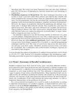
Fig. 7.15 Data dependence
of the Gauss–Seidel and the
SOR method for a
rectangular mesh of size
6 ×4 in the x–y plane. (a)
The data dependences
between the computations of
components are depicted as
arrows between nodes in the
mesh. As an example, for
mesh point 9 the set of nodes
which have to be computed
before point 9 and the set of
nodes which depend on mesh
point 9 are shown. (b)The
data dependences lead to

areas of independent
computations; these are the
diagonals of the mesh from
the upper right to the lower
left. The computations for
mesh points within the same
diagonal can be computed in
parallel. The length of the
diagonals is the degree of
potential parallelism which
can be exploited
123456
789 111210
13 14 15 16 17 18
19 20 21 22 23 24
123456
789
21 24
23
22
20
14
15
16 17
18
121110
13
19
(a) Data dependences of the SOR method
(b) Independent computations within the diagonals

computations for mesh points j > i which are located to the right or below mesh
point i need value x
(k+1)
i
and have to wait for its computation.
The data dependences between computations associated with mesh points are
depicted in the mesh by arrows between the mesh points. It can be observed that
the mesh points in each diagonal from left to right are independent of each other;
these independent mesh points are shown in Fig. 7.15(b). For a square mesh of size
√
n ×
√
n with the same number of mesh points in each dimension, there are at most
√
n independent computations in a single diagonal and at most p =
√
n processors
can be employed.
A parallel implementation can exploit the potential parallelism in a loop structure
with an outer sequential loop and an inner parallel loop. The outer sequential loop
visits the diagonals one after another from the upper left corner to the lower right
corner. The inner loop exploits the parallelism within each diagonal of the mesh.
The number of diagonals is 2
√
n − 1 consisting of
√
n diagonals in the upper left
triangular mesh and
√
n − 1 in the lower triangular mesh. The first

√
n diagonals
l = 1, ,
√
n contain l mesh points i with
i = l + j ·(
√
n − 1) for 0 ≤ j < l .
410 7 Algorithms for Systems of Linear Equations
The last
√
n − 1 diagonals l = 2, ,
√
n contain
√
n −l + 1 mesh points i with
i = l ·
√
n + j ·(
√
n − 1) for 0 ≤ j ≤
√
n −l .
For an implementation on a distributed memory machine, a distribution of the
approximation vector x, the right-hand side b, and the coefficient matrix A is
needed. The elements a
ij
of matrix A are distributed in such a way that the coeffi-
cients for the computation of x
(k+1)

i
according to Formula (7.45) are locally avail-
able. Because the computations are closely related to the mesh, the data distribution
is chosen for the mesh and not the matrix form.
The program fragment with C notation in Fig. 7.16 shows a parallel SPMD
implementation. The data distribution is chosen such that the data associated with
Fig. 7.16 Program fragment of the parallel Gauss–Seidel iteration for a linear equation system
with the banded matrix from the discretized Poisson equation. The computational structure uses
the diagonals of the corresponding discretization mesh, see Fig. 7.15
7.3 Iterative Methods for Linear Systems 411
mesh points in the same mesh row are stored in the same processor. A row-cyclic
distribution of the mesh data is used. The program has two loop nests: The first
loop nest treats the upper diagonals and the second loop nest treats the last diag-
onals. In the inner loops, the processor with name me computes the mesh points
which are assigned to it due to the row-cyclic distribution of mesh points. The
function collect
elements() sends the data computed to the neighboring pro-
cessor, which needs them for the computation of the next diagonal. The function
convergence
test(), not expressed explicitly in this program, can be imple-
mented similarly as in the program in Fig. 7.14 using the maximum norm for
x
(k+1)
− x
(k)
.
The program fragment in Fig. 7.16 uses two-dimensional indices for accessing
array elements of array a. For a large sparse matrix, a storage scheme for sparse
matrices would be used in practice. Also, for a problem such as the discretized
Poisson equation where the coefficients are known it is suitable to code them directly

as constants into the program. This saves expensive array accesses but the code is
less flexible to solve other linear equation systems.
For an implementation on a shared memory machine, the inner loop is performed
in parallel by p =
√
n processors in an SPMD pattern. No data distribution is
needed but the same distribution of work to processors is assigned. Also, no com-
munication is needed to send data to neighboring processors. However, a barrier
synchronization is used instead to make sure that the data of the previous diagonal
are available for the next one.
A further increase of the potential parallelism for solving sparse linear equation
systems can be achieved by the method described in the next section.
7.3.5 Red–Black Ordering
The potential parallelism of the Gauss–Seidel iteration or the successive over-
relaxation for sparse systems resulting from discretization problems can be increased
by an alternative ordering of the unknowns and equations. The goal of the reorder-
ing is to get an equivalent equation system in which more independent compu-
tations exist and, thus, a higher potential parallelism results. The most frequently
used reordering technique is the red–black ordering. The two-dimensional mesh is
regarded as a checkerboard where the points of the mesh represent the squares of the
checkerboard and get corresponding colors. The point (i, j) in the mesh is colored
according to the value of i + j:Ifi + j is even, then the mesh point is red, and if
i + j is odd, then the mesh point is black.
The points in the grid now form two sets of points. Both sets are numbered sep-
arately in a rowwise way from left to right. First the red points are numbered by
1, ,n
R
where n
R
is the number of red points. Then, the black points are numbered

by n
R
+1, ,n
R
+n
B
where n
B
is the number of black points and n = n
R
+n
B
.
The unknowns associated with the mesh points get the same numbers as the mesh
points: There are n
R
unknowns associated with the red points denoted as
ˆ
x
1
, ,
ˆ
x
n
R
and n
B
unknowns associated with the black points denoted as
ˆ
x

n
R
+1
, ,
ˆ
x
n
R
+n
B
.
(The notation
ˆ
x is used to distinguish the new ordering from the original ordering
412 7 Algorithms for Systems of Linear Equations
of the unknowns x. The unknowns are the same as before but their positions in
the system differ.) Figure 7.17 shows a mesh of size 6 × 4 in its original rowwise
numbering in part (a) and a red–black ordering with the new numbering in part (b).
In a linear equation system using red–black ordering, the equations of red
unknowns are arranged before the equations with the black unknown. The equation
system
ˆ
A
ˆ
x =
ˆ
b for the discretized Poisson equation has the form
123456
789 111210
13 14 15 16 17 18

19 20 21 22 23 24
1132 314 15
456
789
16 17 18
19 20 21
22 23 2410 11 12
(a) Mesh in the x−y plane with rowwise numbering
(b) Mesh in the x−y plane with red−black numbering
(c) Matrix structure of the discretized Poisson equation with red−black ordering
Fig. 7.17 Rectangular mesh in the x–y plane of size 6 × 4with(a) rowwise numbering, (b)red–
black numbering, and (c) the matrix of the corresponding linear equation system of the five-point
formula with red–black numbering