7.2 Direct Methods for Linear Systems with Banded Structure 393
for which the values of
˜
a
(k−1)
j
,
˜
b
(k−1)
j
,
˜
c
(k−1)
j
,
˜
y
(k−1)
j
from the previous step computed by a different processor are required. Thus, there
is a communication in each of the log p steps with a message size of four values.
After step N

=log p processor P
i
computes
˜
x
i

=
˜
y
(N

)
i
/
˜
b
(N

)
i
. (7.28)
Phase 3: Parallel substitution of cyclic reduction: After the second phase,
the values
˜
x
i
= x
i·q
are already computed. In this phase, each processor P
i
,
i = 1, ,p, computes the values x
j
with j = (i − 1)q + 1, ,iq − 1in
several steps according to Eq. (7.27). In step k, k = Q − 1, ,0, the elements
x

j
, j = 2
k
, ,n, with step size 2
k+1
are computed. Processor P
i
computes x
j
with
j div q +1 = i for which the values
˜
x
i−1
= x
(i−1)q
and
˜
x
i+1
= x
(i+1)q
computed by
processors P
i−1
and P
i+1
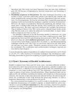
are needed. Figure 7.12 illustrates the parallel algorithm
for p = 2 and n = 8.
i=1

i=3
i=4
i=5
i=6
i=7
i=8
k=0 k=1 k=2 k=3
8
x
4
x
x
x
x
x
x
x
2
6
1
3
5
7
Q steps log p steps Q steps
i=2
phase 1 phase 3phase 2
Fig. 7.12 Illustration of the parallel algorithm for the cyclic reduction for n = 8 equations and
p = 2 processors. Each of the processors is responsible for q = 4 equations; we have Q = 2. The
first and the third phases of the computation have log q = 2 steps. The second phase has log p = 1
step. As recursive doubling is used in the second phase, there are more components of the solution

to be computed in the second phase compared with the computation shown in Fig. 7.11
394 7 Algorithms for Systems of Linear Equations
7.2.2.5 Parallel Execution Time
The execution time of the parallel algorithm can be modeled by the following run-
time functions. Phase 1 executes
Q = log q = log
n
p
= log n −log p
steps where in step k with 1 ≤ k ≤ Q each processor computes at most q/2
k
coefficient blocks of 4 values each. Each coefficient block requires 14 arithmetic
operations according to Eq. (7.23). The computation time of phase 1 can therefore
be estimated as
T
1
(n, p) = 14t
op
·
Q

k=1
q
2
k
≤ 14
n
p
·t
op

.
Moreover, each processor exchanges in each of the Q steps two messages of 4 values
each with its two neighboring processors by participating in single transfer opera-
tions. Since in each step the transfer operations can be performed by all processors
in parallel without interference, the resulting communication time is
C
1
(n, p) = 2Q ·t
s2s
(4) = 2 ·log
n
p
·t
s2s
(4) ,
where t
s2s
(m) denotes the time of a single transfer operation with message size m.
Phase 2 executes log psteps. In each step, each processor computes 4 coefficients
requiring 14 arithmetic operations. Then the value
˜
x
i
= x
i·q
is computed according
to Eq. (7.28) by a single arithmetic operation. The computation time is therefore
T
2
(n, p) = 14log p·t

op
+t
op
.
In each step, each processor sends and receives 4 data values from other processors,
leading to a communication time
C
2
(n, p) = 2log p·t
s2s
(4) .
In each step k of phase 3, k = 0, ,Q−1, each processor computes 2
k
components
of the solution vector according to Eq. (7.27). For each component, five operations
are needed. Altogether, each processor computes

Q−1
k=0
2
k
= 2
Q
− 1 = q − 1
components with one component already computed in phase 2. The resulting com-
putation time is
T
3
(n, p) = 5 ·(q − 1) ·t
op

= 5 ·

n
p
−1

·t
op
.
7.2 Direct Methods for Linear Systems with Banded Structure 395
Moreover, each processor exchanges one data value with each of its neighboring
processors; the communication time is therefore
C
3
(n, p) = 2 ·t
s2s
(1) .
The resulting total computation time is
T (n, p) =

14
n
p
+14 ·log p+5
n
p
−4

· t
op



19
n
p
+14 ·log p

· t
op
.
The communication overhead is
C(n, p) =

2 · log
n
p
+2log p

t
s2s
(4) + 2 ·t
s2s
(1)
 2 ·log n ·t
s2s
(4) + 2 ·t
s2s
(1) .
Compared to the sequential algorithm, the parallel implementation leads to a small
computational redundancy of 14 · log p operations. The communication overhead

increases logarithmically with the number of rows, whereas the computation time
increases linearly.
7.2.3 Generalization to Banded Matrices
The cyclic reduction algorithm can be generalized to banded matrices with semi-
bandwidth r > 1. For the description we assume n = s ·r. The matrix is represented
as a block-tridiagonal matrix of the form
⎛
⎜
⎜
⎜
⎜
⎜
⎜
⎝
B
(0)
1
C
(0)
1
0
A
(0)
2
B
(0)
2
C
(0)
2

.
.
.
.
.
.
.
.
.
A
(0)
s−1
B
(0)
s−1
C
(0)
s−1
0 A
(0)
s
B
(0)
s
⎞
⎟
⎟
⎟
⎟
⎟

⎟
⎠
⎛
⎜
⎜
⎜
⎜
⎜
⎝
X
1
X
2
.
.
.
X
s−1
X
s
⎞
⎟
⎟
⎟
⎟
⎟
⎠
=
⎛
⎜

⎜
⎜
⎜
⎜
⎜
⎝
Y
(0)
1
Y
(0)
2
.
.
.
Y
(0)
s−1
Y
(0)
s
⎞
⎟
⎟
⎟
⎟
⎟
⎟
⎠
,

where
A
(0)
i
= (a
lm
)
l∈I
i
,m∈I
i−1
for i = 2, ,s ,
B
(0)
i
= (a
lm
)
l∈I
i
,m∈I
i
for i = 1, ,s ,
C
(0)
i
= (a
lm
)
l∈I

i
,m∈I
i+1
for i = 1, ,s −1
are sub-matrices of A. The index sets are for i = 1, ,s
I
i
={j ∈ N | (i − 1)r < j ≤ ir}.
396 7 Algorithms for Systems of Linear Equations
The vectors X
i
, Y
(0)
i
∈ R
r
are
X
i
= (x
l
)
l∈I
i
and Y
(0)
i
= (y
l
)

l∈I
i
for i = 1, ,s.
The algorithm from above is generalized by applying the described computation
steps for elements according to Eq. (7.23) to blocks and using matrix operations
instead of operations on single elements. In the first step, three consecutive matrix
equations i −1, i, i + 1fori = 3, 4, ,s −2 are considered:
A
(0)
i−1
X
i−2
+B
(0)
i−1
X
i−1
+ C
(0)
i−1
X
i
=Y
(0)
i−1
,
A
(0)
i
X

i−1
+ B
(0)
i
X
i
+ C
(0)
i
X
i+1
=Y
(0)
i
,
A
(0)
i+1
X
i
+B
(0)
i+1
X
i+1
+C
(0)
i+1
X
i+2

=Y
(0)
i+1
.
Equation (i − 1) is used to eliminate subvector X
i−1
from equation i and equation
(i + 1) is used to eliminate subvector X
i+1
from equation i. The algorithm starts
with the following initializations:
A
(0)
1
:= 0 ∈ R
r×r
, C
(0)
s
:= 0 ∈ R
r×r
and for k = 0, ,log sand i ∈ Z \{1, ,s}
A
(k)
i
= C
(k)
i
:= 0 ∈ R
r×r

,
B
(k)
i
:= I ∈ R
r×r
,
Y
(k)
i
:= 0 ∈ R
r
.
In step k = 1, ,log sthe following sub-matrices
α
(k)
i
:=−A
(k−1)
i

B
(k−1)
i−2
k−1

−1
,
β
(k)

i
:=−C
(k−1)
i

B
(k−1)
i+2
k−1

−1
,
A
(k)
i
= α
(k)
i
· A
(k−1)
i−2
k−1
,
C
(k)
i
= β
(k)
i
·C

(k−1)
i+2
k−1
, (7.29)
B
(k)
i
= α
(k)
i
C
(k−1)
i−2
k−1
+ B
(k−1)
i
+β
(k)
i
A
(k−1)
i+2
k−1
and the vector
Y
(k)
i
= α
(k)

i
Y
(k−1)
i−2
k−1
+Y
(k−1)
i
+β
(k)
i
Y
(k−1)
i+2
k−1
(7.30)
are computed. The resulting matrix equations are
7.2 Direct Methods for Linear Systems with Banded Structure 397
A
(k)
i
X
i−2
k
+ B
(k)
i
X
i
+C

(k)
i
X
i+2
k
= Y
(k)
i
(7.31)
for i = 1, ,s. In summary, the method of cyclic reduction for banded matrices
comprises the following two phases:
1. Elimination phase: For k = 1, ,log scompute the matrices A
(k)
i
, B
(k)
i
, C
(k)
i
and the vector Y
(k)
i
for i = 2
k
, ,s with step size 2
k
according to Eqs. (7.29)
and (7.30).
2. Substitution phase: For k =log s, ,0 compute subvector X

i
for i =
2
k
, ,s with step size 2
k+1
by solving the linear equation system (7.31), i.e.,
B
(k)
i
X
i
= Y
(k)
i
− A
(k)
i
X
i−2
k
−C
(k)
i
X
i+2
k
.
The computation of α
(k)

i
and β
(k)
i
requires a matrix inversion or the solution of
a dense linear equation system with a direct method requiring O(r
3
) computations,
i.e., the computations increase with the bandwidth cubically. The first step requires
the computation of O(s) = O(n/r) sub-matrices; the asymptotic runtime for this
step is therefore O(nr
2
). The second step solves a total number of O(s) = O(n/r)
linear equation systems, also resulting in an asymptotic runtime of O(nr
2
).
For the parallel implementation of the cyclic reduction for banded matrices, the
parallel method described for tridiagonal systems with its three phases can be used.
The main difference is that arithmetic operations in the implementation for tridiag-
onal systems are replaced by matrix operations in the implementation for banded
systems, which increases the amount of computations for each processor. The com-
putational effort for the local operations is now O(r
3
). Also, the communication
between the processors exchanges larger messages. Instead of single numbers, entire
matrices of size r × r are exchanged so that the message size is O(r
2
). Thus,
with growing semi-bandwidth r of the banded matrix the time for the computa-
tion increases faster than the communication time. For p  s an efficient parallel

implementation can be expected.
7.2.4 Solving the Discretized Poisson Equation
The cyclic reduction algorithm for banded matrices presented in Sect. 7.2.3 is
suitable for the solution of the discretized two-dimensional Poisson equation. As
shown in Sect. 7.2.1, this linear equation system has a banded structure with
semi-bandwidth N where N is the number of discretization points in the x-or
y-dimension of the two-dimensional domain, see Fig. 7.9. The special structure has
only four non-zero diagonals and the band has a sparse structure. The use of the
Gaussian elimination method would not preserve the sparse banded structure of the
matrix, since the forward elimination for eliminating the two lower diagonals leads
to fill-ins with non-zero elements between the two upper diagonals. This induces a
higher computational effort which is needed for banded matrices with a dense band
of semi-bandwidth N. In the following, we consider the method of cyclic reduction
for banded matrices, which preserves the sparse banded structure.
398 7 Algorithms for Systems of Linear Equations
The blocks of the discretized Poisson equation Az = d for a representation as
blocked tridiagonal matrix are given by Eqs. (7.18) and (7.19). Using the notation
for the banded system, we get
B
(0)
i
:=
1
h
2
B for i = 1, ,N ,
A
(0)
i
:=−

1
h
2
I and C
(0)
i
:=−
1
h
2
I for i = 1, ,N .
The vector d ∈ R
n
consists of N subvectors D
j
∈ R
N
, i.e.,
d =
⎛
⎜
⎝
D
1
.
.
.
D
N
⎞

⎟
⎠
with D
j
=
⎛
⎜
⎝
d
( j−1)N+1
.
.
.
d
jN
⎞
⎟
⎠
.
Analogously, the solution vector consists of N subvectors Z
j
of length N each, i.e.,
z =
⎛
⎜
⎝
Z
1
.
.

.
Z
N
⎞
⎟
⎠
with Z
j
=
⎛
⎜
⎝
z
( j−1)N+1
.
.
.
z
j·N
⎞
⎟
⎠
.
The initialization for the cyclic reduction algorithm is given by
B
(0)
:= B ,
D
(0)
j

:= D
j
for j = 1, ,N ,
D
(k)
j
:= 0fork = 0, ,log N, j ∈ Z \{1, ,N} ,
Z
j
:= 0forj ∈ Z \{1, ,N} .
In step k of the cyclic reduction, k = 1, ,log N, the matrices B
(k)
∈ R
N×N
and
the vectors D
(k)
j
∈ R
N
for j = 1, ,N are computed according to
B
(k)
= (B
(k−1)
)
2
−2I ,
D
(k)

j
= D
(k−1)
j−2
k−1
+ B
(k−1)
D
(k−1)
j
+ D
(k−1)
j+2
k−1
. (7.32)
For k = 0, ,log N Eq. (7.31) has the special form
− Z
j−2
k
+ B
(k)
Z
j
− Z
j+2
k
= D
(k)
j
for j = 1, ,n . (7.33)

Together Eqs. (7.32) and (7.33) represent the method of cyclic reduction for the
discretized Poisson equation, which can be seen by induction. For k = 0, Eq. (7.33)
is the initial equation system Az = d.For0< k < log N and j ∈{1, ,N} the
three equations
7.3 Iterative Methods for Linear Systems 399
−Z
j−2
k+1
+B
(k)
Z
j−2
k
− Z
j
=D
(k)
j−2
k
,
− Z
j−2
k
+B
(k)
Z
j
− Z
j+2
k

= D
(k)
j
,
− Z
j
+B
(k)
Z
j+2
k
−Z
j+2
k+1
= D
(k)
j+2
k
(7.34)
are considered. The multiplication of Eq. (7.33) with B
(k)
from the left results in
− B
(k)
Z
j−2
k
+ B
(k)
B

(k)
Z
j
− B
(k)
Z
j+2
k
= B
(k)
D
(k)
j
. (7.35)
Adding Eq. (7.35) with the first part in Eq. (7.34) and the third part in Eq. (7.34)
results in
−Z
j−2
k+1
− Z
j
+B
(k)
B
(k)
Z
j
− Z
j
−Z

j+2
k+1
= D
(k)
j−2
k
+ B
(k)
D
(k)
j
+ D
(k)
j+2
k
,
which shows that Formula (7.32) for k +1 is derived. In summary, the cyclic reduc-
tion for the discretized two-dimensional Poisson equation consists of the following
two steps:
1. Elimination phase: For k = 1, ,log N, the matrices B
(k)
and the vectors
D
(k)
j
are computed for j = 2
k
, ,N with step size 2
k
according to Eq. (7.32).

2. Substitution phase: For k =log N, ,0, the linear equation system
B
(k)
Z
j
= D
(k)
j
+ Z
j−2
k
+ Z
j+2
k
for j = 2
k
, ,N with step size 2
k+1
is solved.
In the first phase, log N matrices and O(N) subvectors are computed. The com-
putation of each matrix includes a matrix multiplication with time O(N
3
). The
computation of a subvector includes a matrix–vector multiplication with complexity
O(N
2
). Thus, the first phase has a computational complexity of O(N
3
log N). In the
second phase, O(N) linear equation systems are solved. This requires time O(N

3
)
when the special structure of the matrices B
(k)
is not exploited. In [61] it is shown
how to reduce the time by exploiting this structure. A parallel implementation of
the discretized Poisson equation can be done in an analogous way as shown in the
previous section.
7.3 Iterative Methods for Linear Systems
In this section, we introduce classical iteration methods for solving linear equa-
tion systems, including the Jacobi iteration, the Gauss–Seidel iteration, and the
SOR method (successive over-relaxation), and discuss their parallel implementa-
tion. Direct methods as presented in the previous sections involve a factorization
of the coefficient matrix. This can be impractical for large and sparse matrices,
since fill-ins with non-zero elements increase the computational work. For banded
400 7 Algorithms for Systems of Linear Equations
matrices, special methods can be adapted and used as discussed in Sect. 7.2. Another
possibility is to use iterative methods as presented in this section.
Iterative methods for solving linear equation systems Ax = b with coefficient
matrix A ∈ R
n×n
and right-hand side b ∈ R
n
generate a sequence of approximation
vectors {x
(k)
}
k=1,2,
that converges to the solution x
∗

∈ R
n
. The computation of an
approximation vector essentially involves a matrix–vector multiplication with the
iteration matrix of the specific problem. The matrix A of the linear equation system
is used to build this iteration matrix. For the evaluation of an iteration method it is
essential how quickly the iteration sequence converges. Basic iteration methods are
the Jacobi and the Gauss–Seidel methods, which are also called relaxation methods
historically, since the computation of a new approximation depends on a combina-
tion of the previously computed approximation vectors. Depending on the specific
problem to be solved, relaxation methods can be faster than direct solution methods.
But still these methods are not fast enough for practical use. A better convergence
behavior can be observed for methods like the SOR method, which has a similar
computational structure. The practical importance of relaxation methods is their use
as preconditioner in combination with solution methods like the conjugate gradient
method or the multigrid method. Iterative methods are a good first example to study
parallelism as it is typical also for more complex iteration methods. In the following,
we describe the relaxation methods according to [23], see also [71, 166]. Parallel
implementations are considered in [60, 61, 72, 154].
7.3.1 StandardIteration Methods
Standard iteration methods for the solution of a linear equation system Ax = b are
based on a splitting of the coefficient matrix A ∈ R
n×n
into
A = M − N with M, N ∈ R
n×n
,
where M is a non-singular matrix for which the inverse M
−1
can be computed easily,

e.g., a diagonal matrix. For the unknown solution x
∗
of the equation Ax = b we get
Mx
∗
= Nx
∗
+b .
This equation induces an iteration of the form Mx
(k+1)
= Nx
(k)
+b, which is usually
written as
x
(k+1)
= Cx
(k)
+d (7.36)
with iteration matrix C := M
−1
N and vector d := M
−1
b. The iteration method is
called convergent if the sequence {x
(k)
}
k=1,2,
converges toward x
∗

independently
of the choice of the start vector x
(0)
∈ R
n
, i.e., lim
k→∞
x
(k)
= x
∗
or lim
k→∞
x
(k)
−
x
∗
=0. When a sequence converges the vector x
∗
is uniquely defined by x
∗
=
Cx
∗
+d. Subtracting this equation from Eq. (7.36) and using induction leads to the
7.3 Iterative Methods for Linear Systems 401
equality x
(k)
− x

∗
= C
k
(x
(0)
− x
∗
), where C
k
denotes the matrix resulting from k
multiplications of C. Thus, the convergence of Eq. (7.36) is equivalent to
lim
k→∞
C
k
= 0 .
A result from linear algebra shows the relation between the convergence criteria
and the spectral radius ρ(C) of the iteration matrix C. (The spectral radius of a
matrix is the eigenvalue with the largest absolute value, i.e., ρ(C) = max
λ∈EW
|λ| with
EW ={λ |Cv = λv, v = 0}.) The following properties are equivalent, see [166]:
(1) Iteration (7.36) converges for every x
(0)
∈ R
n
.
(2) lim
k→∞
C

k
= 0.
(3) ρ(C) < 1.
Well-known iteration methods are the Jacobi, the Gauss–Seidel, and the SOR
method.
7.3.1.1 Jacobi Iteration
The Jacobi iteration is based on the splitting A = D − L − R of the matrix A with
D, L, R ∈ R
n×n
. The matrix D holds the diagonal elements of A, −L holds the
elements of the lower triangular of A without the diagonal elements, and −R holds
the elements of the upper triangular of A without the diagonal elements. All other
elements of D, L, R are zero. The splitting is used for an iteration of the form
Dx
(k+1)
= (L + R)x
(k)
+b,
which leads to the iteration matrix C
Ja
:= D
−1
(L + R)or
C
Ja
= (c
ij
)
i, j=1, ,n
with c

ij
=

−a
ij
/a
ii
for j = i ,
0 otherwise .
The matrix form is used for the convergence proof, not shown here. For the practical
computation, the equation written out with all its components is more suitable:
x
(k+1)
i
=
1
a
ii
⎛
⎝
b
i
−
n

j=1, j=i
a
ij
x
(k)

j
⎞
⎠
, i = 1, ,n . (7.37)
The computation of one component x
(k+1)
i
, i ∈{1, ,n},ofthe(k + 1)th approx-
imation requires all components of the kth approximation vector x
k
. Considering a
sequential computation in the order x
(k+1)
1
, ,x
(k+1)
n
, it can be observed that the
values x
(k+1)
1
, ,x
(k+1)
i−1
are already known when x
(k+1)
i
is computed. This informa-
tion is exploited in the Gauss–Seidel iteration method.
402 7 Algorithms for Systems of Linear Equations

7.3.1.2 Gauss–Seidel Iteration
The Gauss–Seidel iteration is based on the same splitting of the matrix A as the
Jacobi iteration, i.e., A = D − L − R, but uses the splitting in a different way for
an iteration
(D − L)x
(k+1)
= Rx
(k)
+b .
Thus, the iteration matrix of the Gauss–Seidel method is C
Ga
:= (D − L)
−1
R;this
form is used for numerical properties like convergence proofs, not shown here. The
component form for the practical use is
x
(k+1)
i
=
1
a
ii
⎛
⎝
b
i
−
i−1


j=1
a
ij
x
(k+1)
j
−
n

j=i+1
a
ij
x
(k)
j
⎞
⎠
, i = 1, ,n . (7.38)
It can be seen that the components of x
(k+1)
i
, i ∈{1, ,n}, uses the new infor-
mation x
(k+1)
1
, ,x
(k+1)
i−1
already determined for that approximation vector. This is
useful for a faster convergence in a sequential implementation, but the potential

parallelism is now restricted.
7.3.1.3 Convergence Criteria
For the Jacobi and the Gauss–Seidel iteration the following convergence criteria
based on the structure of A is often helpful. The Jacobi and the Gauss–Seidel itera-
tion converge if the matrix A is strongly diagonal dominant, i.e.,
|a
ii
| >
n

j=1, j=i
|a
ij
| , i = 1, ,n .
When the absolute values of the diagonal elements are large compared to the sum
of the absolute values of the other row elements, this often leads to a better conver-
gence. Also, when the iteration methods converge, the Gauss–Seidel iteration often
converges faster than the Jacobi iteration, since always the most recently computed
vector components are used. Still the convergence is usually not fast enough for
practical use. Therefore, an additional relaxation parameter is introduced to speed
up the convergence.
7.3.1.4 JOR Method
The JOR method or Jacobi over-relaxation is based on the splitting A =
1
ω
D −L −
R −
1−ω
ω
D of the matrix A with a relaxation parameter ω ∈ R. The component

form of this modification of the Jacobi method is