352 6 Thread Programming
Besides the explicit flush construct there is an implicit flush at several points
of the program code, which are
• a barrier construct;
• entry to and exit from a critical region;
• at the end of a parallel region;
• at the end of a for, sections,orsingle construct without nowait clause;
• entry and exit of lock routines (which will be introduced below).
6.3.3.1 Locking Mechanism
The OpenMP runtime system also provides runtime library functions for a synchro-
nization of threads with the locking mechanism. The locking mechanism has been
described in Sect. 4.3 and in this chapter for Pthreads and Java threads. The specific
locking mechanism of the OpenMP library provides two kinds of lock variables
on which the locking runtime routines operate. Simple locks of type omp
lock t
can be locked only once. Nestable locks of type omp
nest lock t can be locked
multiple times by the same thread. OpenMP lock variables should be accessed only
by OpenMP locking routines. A lock variable is initialized by one of the following
initialization routines:
void omp
init lock (omp lock t
*
lock)
void omp
init nest lock (omp nest lock t
*
lock)
for simple and nestable locks, respectively. A lock variable is removed with the
routines
void omp

destroy lock (omp lock t
*
lock)
void omp
destroy nest lock (omp nest lock t
*
lock).
An initialized lock variable can be in the states locked or unlocked. At the begin-
ning, the lock variable is in the state unlocked. A lock variable can be used for the
synchronization of threads by locking and unlocking. To lock a lock variable the
functions
void omp
set lock (omp lock t
*
lock)
void omp
set nest lock (omp nest lock t
*
lock)
are provided. If the lock variable is available, the thread calling the lock routine
locks the variable. Otherwise, the calling thread blocks. A simple lock is available
when no other thread has locked the variable before without unlocking it. A nestable
lock variable is available when no other thread has locked the variable without
unlocking it or when the calling thread has locked the variable, i.e., multiple locks
for one nestable variable by the same thread are possible counted by an internal
counter. When a thread uses a lock routine to lock a variable successfully, this thread
6.4 Exercises for Chap. 6 353
is said to own the lock variable. A thread owning a lock variable can unlock this
variable with the routines
void omp

unset lock (omp lock t
*
lock)
void omp
unset nest lock (omp nest lock t
*
lock).
For a nestable lock, the routine omp
unset nest lock () decrements the inter-
nal counter of the lock. If the counter has the value 0 afterwards, the lock variable
is in the state unlocked. The locking of a lock variable without a possible blocking
of the calling thread can be performed by one of the routines
void omp
test lock (omp lock t
*
lock)
void omp
test nest lock (omp nest lock t
*
lock)
for simple and nestable lock variables, respectively. When the lock is available, the
routines lock the variable or increment the internal counter and return a result value
= 1. When the lock is not available, the test routine returns 0 and the calling
thread is not blocked.
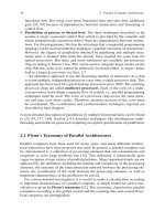
Example Figure 6.50 illustrates the use of nestable lock variables, see [130]. A
data structure pair consists of two integers a and b and a nestable lock vari-
able l, which is used to synchronize the updates of a, b, or the entire pair.
It is assumed that the lock variable l has been initialized before calling f().The
increment functions incr
a() for incrementing a, incr b() for incrementing b,

and incr
pair() for incrementing both integer variables are given. The function
incr
a() is only called from incr pair() and does not need an additional
locking. The functions incr
b() and incr pair() are protected by the lock
since they can be called concurrently. 
6.4 Exercises for Chap. 6
Exercise 6.1 Modify the matrix multiplication program from Fig. 6.1 on p. 262 so
that a fixed number of threads is used for the multiplication of matrices of arbitrary
size. For the modification, let each thread compute the rows of the result matrix
instead of a single entry. Compute the number of rows that each thread must com-
pute such that each thread has about the same number of rows to compute. Is there
any synchronization required in the program?
Exercise 6.2 Use the task pool implementation from Sect. 6.1.6 on p. 276 to imple-
ment a parallel matrix multiplication. To do so, use the function thread
mult()
from Fig. 6.1 to define a task as the computation of one entry of the result matrix
and modify the function if necessary so that it fits to the requirements of the task
pool. Modify the main program so that all tasks are generated and inserted into the
task pool before the threads to perform the computations are started. Measure the
354 6 Thread Programming
Fig. 6.50 Program fragment
illustrating the use of nestable
lock variables
resulting execution time for different numbers of threads and different matrix sizes
and compare the execution time with the execution time of the implementation of
the last exercise.
Exercise 6.3 Consider the r/w lock mechanism in Fig. 6.5. The implementation
given does not provide operations that are equivalent to the function

pthread mutex
trylock(). Extend the implementation from Fig. 6.5 by specifying functions
rw
lock rtrylock() and rw lock wtrylock() which return EBUSY if the
requested read or write permit cannot be granted.
Exercise 6.4 Consider the r/w lock mechanism in Fig. 6.5. The implementation
given favors read requests over write requests in the sense that a thread will get
a write permit only if no other thread requests a read permit, but read permits
are given without waiting also in the presence of other read permits. Change the
implementation such that write permits have priority, i.e., as soon as a write permit
6.4 Exercises for Chap. 6 355
arrives, no more read permits are granted until the write permit has been granted and
the corresponding write operation is finished. To test the new implementation write
a program which starts three threads, two read threads, and one write thread. The
first read thread requests five read permits one after another. As soon as it gets the
read permits it prints a control message and waits for 2 s (use sleep(2)) before
requesting the next read permit. The second read thread does the same except that
it only waits 1 s after the first read permit and 2 s otherwise. The write thread first
waits 5 s and then requests a write permit and prints a control message after it has
obtained the write permit; then the write permit is released again immediately.
Exercise 6.5 An r/w lock mechanism allows multiple readers to access a data struc-
ture concurrently, but only a single writer is allowed to access the data structures at
a time. We have seen a simple implementation of r/w locks in Pthreads in Fig. 6.5.
Transfer this implementation to Java threads by writing a new class RWlock with
entries num
r and num w to count the current number of read and write permits
given. The class RWlock should provide methods similar to the functions in Fig. 6.5
to request or release a read or write permit.
Exercise 6.6 Consider the pipelining programming pattern and its Pthreads imple-
mentation in Sect. 6.1.7. In the example given, each pipeline stage adds 1 to the

integer value received from the predecessor stage. Modify the example such that
pipeline stage i adds the value i to the value received from the predecessor. In the
modification, there should still be only one function pipe
stage() expressing
the computations of a pipeline stage. This function must receive an appropriate
parameter for the modification.
Exercise 6.7 Use the task pool implementation from Sect. 6.1.6 to define a parallel
loop pattern. The loop body should be specified as function with the loop variable as
parameter. The iteration space of the parallel loop is defined as the set of all values
that the loop variable can have. To execute a parallel loop, all possible indices are
stored in a parallel data structure similar to a task pool which can be accessed by all
threads. For the access, a suitable synchronization must be used.
(a) Modify the task pool implementation accordingly such that functions for the
definition of a parallel loop and for retrieving an iteration from the parallel loop
are provided. The thread function should also be provided.
(b) The parallel loop pattern from (a) performs a dynamic load balancing since a
thread can retrieve the next iteration as soon as its current iteration is finished.
Modify this operation such that a thread retrieves a chunk of iterations instead
of a single operation to reduce the overhead of load balancing for fine-grained
iterations.
(c) Include guided self-scheduling (GSS) in your parallel loop pattern. GSS adapts
the number of iterations retrieved by a thread to the total number of iterations
that are still available. If n threads are used and there are R
i
remaining iterations,
the next thread retrieves
356 6 Thread Programming
x
i
=


R
i
n

iterations, i = 1, 2, . For the next retrieval, R
i+1
= R
i
− x
i
iterations remain.
R
1
is the initial number of iterations to be executed.
(d) Use the parallel loop pattern to express the computation of a matrix multiplica-
tion where the computation of each matrix entry can be expressed as an iteration
of a parallel loop. Measure the resulting execution time for different matrix
sizes. Compare the execution time for the two load balancing schemes (standard
and GSS) implemented.
Exercise 6.8 Consider the client–server pattern and its Pthreads implementation in
Sect. 6.1.8. Extend the implementation given in this section by allowing a cancel-
lation with deferred characteristics. To be cancellation-safe, mutex variables that
have been locked must be released again by an appropriate cleanup handler. When
a cancellation occurs, allocated memory space should also be released. In the server
function tty
server routine(), the variable running should be reset when
a cancellation occurs. Note that this may create a concurrent access. If a cancellation
request arrives during the execution of a synchronous request of a client, the client
thread should be informed that a cancellation has occurred. For a cancellation in the

function client
routine(), the counter client threads should be kept
consistent.
Exercise 6.9 Consider the task pool pattern and its implementation in Pthreads in
Sect. 6.1.6. Implement a Java class TaskPool with the same functionality. The
task pool should accept each object of a class which implements the interface
Runnable as task. The tasks should be stored in an array final Runnable
tasks[]. A constructor TaskPool(int p, int n) should be implemented
that allocates a task array of size n and creates p threads which access the task
pool. The methods run() and insert(Runnable w) should be implemented
according to the Pthreads functions tpool
thread() and tpool insert()
from Fig. 6.7. Additionally, a method terminate() should be provided to termi-
nate the threads that have been started in the constructor. For each access to the task
pool, a thread should check whether a termination request has been set.
Exercise 6.10 Transfer the pipelining pattern from Sect. 6.1.7 for which Figs. 6.8,
6.9, 6.10, and 6.11 give an implementation in Pthreads to Java. For the Java imple-
mentation, define classes for a pipeline stage as well as for the entire pipeline which
provide the appropriate method to perform the computation of a pipeline stage, to
send data into the pipeline, and to retrieve a result from the last stage of the pipeline.
Exercise 6.11 Transfer the client–server pattern for which Figs. 6.13, 6.14, 6.15,
and 6.16 give a Pthreads implementation to Java threads. Define classes to store a
request and for the server implementation explain the synchronizations performed
and give reasons that no deadlock can occur.
Exercise 6.12 Consider the following OpenMP program piece:
6.4 Exercises for Chap. 6 357
int x=0;
int y=0;
void foo1() {
#pragma omp critical (x)

{ foo2(); x+=1; }
}
void foo2() {
#pragma omp critical(y)
{ y+=1; }
}
void foo3() {
#pragma omp critical(y)
{ y-=1; foo4(); }
}
void foo4() {
#pragma omp critical(x)
{ x-=1; }
}
int main(int argx, char
**
argv) {
int x;
#pragma omp parallel private(i) {
for (i=0; i<10; i++)
{ foo1(), foo3(); }
}
printf(’’%d %d \n’’, x,y )
}
We assume that two threads execute this piece of code on two cores of a multicore
processor. Can a deadlock situation occur? If so, describe the execution order which
leads to the deadlock. If not, give reasons why a deadlock is not possible.
Chapter 7
Algorithms for Systems of Linear Equations
The solution of a system of simultaneous linear equations is a fundamental problem

in numerical linear algebra and is a basic ingredient of many scientific simulations.
Examples are scientific or engineering problems modeled by ordinary or partial dif-
ferential equations. The numerical solution is often based on discretization methods
leading to a system of linear equations. In this chapter, we present several standard
methods for solving systems of linear equations of the form
Ax = b, (7.1)
where A ∈ R
n×n
is an (n × n) matrix of real numbers, b ∈ R
n
is a vector of
size n, and x ∈ R
n
is an unknown solution vector of size n specified by the lin-
ear system (7.1) to be determined by a solution method. There exists a solution x
forEq.(7.1)ifthematrixA is non-singular, which means that a matrix A
−1
with
A · A
−1
= I exists; I denotes the n-dimensional identity matrix and · denotes the
matrix product. Equivalently, the determinant of matrix A is not equal to zero. For
the exact mathematical properties we refer to a standard book for linear algebra
[71]. The emphasis of the presentation in this chapter is on parallel implementation
schemes for linear system solvers.
The solution methods for linear systems are classified as direct and iterative.
Direct solution methods determine the exact solution (except rounding errors) in a
fixed number of steps depending on the size n of the system. Elimination methods
and factorization methods are considered in the following. Iterative solution meth-
ods determine an approximation of the exact solution. Starting with a start vector, a

sequence of vectors is computed which converges to the exact solution. The compu-
tation is stopped if the approximation has an acceptable precision. Often, iterative
solution methods are faster than direct methods and their parallel implementation
is straightforward. On the other hand, the system of linear equations needs to fulfill
some mathematical properties in order to guarantee the convergence to the exact
solution. For sparse matrices, in which many entries are zeros, there is an advantage
for iterative methods since they avoid a fill-in of the matrix with non-zero elements.
This chapter starts with a presentation of Gaussian elimination, a direct solver,
and its parallel implementation with different data distribution patterns. In Sect. 7.2,
direct solution methods for linear systems with tridiagonal structure or banded
T. Rauber, G. R
¨
unger, Parallel Programming,
DOI 10.1007/978-3-642-04818-0
7,
C

Springer-Verlag Berlin Heidelberg 2010
359
360 7 Algorithms for Systems of Linear Equations
matrices, in particular cyclic reduction and recursive doubling, are discussed.
Section 7.3 is devoted to iterative solution methods, Sect. 7.5 presents the Cholesky
factorization, and Sect. 7.4 introduces the conjugate gradient method. All presenta-
tions mainly concentrate on the aspects of a parallel implementation.
7.1 Gaussian Elimination
For the well-known Gaussian elimination, we briefly present the sequential method
and then discuss parallel implementations with different data distributions. The
section closes with an analysis of the parallel runtime of the Gaussian elimination
with double-cyclic data distribution.
7.1.1 Gaussian Elimination and LU Decomposition

Written out in full the linear system Ax = b has the form
a
11
x
1
+ a
12
x
2
+···+a
1n
x
n
= b
1
.
.
.
.
.
.
.
.
.
.
.
.
a
i1
x

1
+ a
i2
x
2
+···+a
in
x
n
= b
i
.
.
.
.
.
.
.
.
.
.
.
.
a
n1
x
1
+ a
n2
x

2
+···+a
nn
x
n
= b
n
.
The Gaussian elimination consists of two phases, the forward elimination and the
backward substitution. The forward elimination transforms the linear system (7.1)
into a linear system Ux = b

with an (n ×n)matrixU in upper triangular form. The
transformation employs reordering of equations or operations that add a multiple of
one equation to another. Hence, the solution vector remains unchanged. In detail, the
forward elimination performs the following n − 1 steps. The matrix A
(1)
:= A =
(a
ij
) and the vector b
(1)
:= b = (b
i
) are subsequently transformed into matrices
A
(2)
, ,A
(n)
and vectors b

(2)
, ,b
(n)
, respectively. The linear equation systems
A
(k)
x = b
(k)
have the same solution as Eq. (7.1) for k = 2, ,n. The matrix A
(k)
computed in step k −1 has the form
A
(k)
=
⎡
⎢
⎢
⎢
⎢
⎢
⎢
⎢
⎢
⎢
⎢
⎢
⎢
⎢
⎣
a

11
a
12
··· a
1,k−1
a
1k
··· a
1n
0 a
(2)
22
··· a
(2)
2,k−1
a
(2)
2k
··· a
(2)
2n
.
.
.
.
.
.
.
.
.

.
.
.
.
.
.
.
.
.
.
.
.
.
.
.
a
(k−1)
k−1,k−1
a
(k−1)
k−1,k
··· a
(k−1)
k−1,n
.
.
.0a
(k)
kk
··· a

(k)
kn
.
.
.
.
.
.
.
.
.
.
.
.
.
.
.
0 ··· ··· 0 a
(k)
nk
··· a
(k)
nn
⎤
⎥
⎥
⎥
⎥
⎥
⎥

⎥
⎥
⎥
⎥
⎥
⎥
⎥
⎦
.
7.1 Gaussian Elimination 361
The first k − 1 rows are identical to the rows in matrix A
(k−1)
. In the first k − 1
columns, all elements below the diagonal element are zero. Thus, the last matrix
A
(n)
has upper triangular form. The matrix A
(k+1)
and the vector b
(k+1)
are cal-
culated from A
(k)
and b
(k)
, k = 1, ,n − 1, by subtracting suitable multiples
of row k of A
(k)
and element k of b
(k)

from the rows k + 1, k + 2, ,n of
A and elements b
(k)
k+1
, b
(k)
k+2
, ,b
(k)
n
, respectively. The elimination factors for row
i are
l
ik
= a
(k)
ik
/a
(k)
kk
, i = k + 1, ,n . (7.2)
They are chosen such that the coefficient of x
k
of the unknown vector x is eliminated
from equations k +1, k + 2, ,n. The rows of A
(k+1)
and the entries of b
(k+1)
are
calculated according to

a
(k+1)
ij
= a
(k)
ij
−l
ik
a
(k)
kj
, (7.3)
b
(k+1)
i
= b
(k)
i
−l
ik
b
(k)
k
(7.4)
for k < j ≤ n and k < i ≤ n. Using the equation system A
(n)
x = b
(n)
, the result
vector x is calculated in the backward substitution in the order x

n
, x
n−1
, ,x
1
according to
x
k
=
1
a
(n)
kk
⎛
⎝
b
(n)
k
−
n

j=k+1
a
(n)
kj
x
j
⎞
⎠
. (7.5)

Figure 7.1 shows a program fragment in C for a sequential Gaussian elimination.
The inner loop computing the matrix elements is iterated approximately k
2
times so
that the entire loop has runtime

n
k=1
k
2
=
1
6
n(n +1)(2n + 1) ≈ n
3
/3 which leads
to an asymptotic runtime O(n
3
).
7.1.1.1 LU Decomposition and Triangularization
The matrix A can be represented as the matrix product of an upper triangular matrix
U := A
(n)
and a lower triangular matrix L which consists of the elimination factors
(7.2) in the following way:
L =
⎡
⎢
⎢
⎢

⎢
⎢
⎣
100 0
l
21
10 0
l
31
l
32
10
.
.
.
.
.
.
.
.
.
.
.
.
0
l
n1
l
n2
l

n3
l
n,n−1
1
⎤
⎥
⎥
⎥
⎥
⎥
⎦
.
The matrix representation A = L ·U is called triangularization or LU decompo-
sition. When only the LU decomposition is needed, the right-hand side of the linear
362 7 Algorithms for Systems of Linear Equations
Fig. 7.1 Program fragment in C notation for a sequential Gaussian elimination of the linear system
Ax = b.ThematrixA is stored in array a, the vector b is stored in array b. The indices start
with 0. The functions max
col(a,k) and exchange row(a,b,r,k) implement pivoting.
The function max
col(a,k) returns the index r with |a
rk
|=max
k≤s≤n
(|a
sk
|). The function
exchange
row(a,b,r,k) exchanges the rows r and k of A and the corresponding elements
b

r
and b
k
of the right-hand side
system does not have to be transformed. Using the LU decomposition, the linear
system Ax = b can be rewritten as
Ax = LA
(n)
x = Ly = b with y = A
(n)
x (7.6)
and the solution can be determined in two steps. In the first step, the vector y is
obtained by solving the triangular system Ly = b by forward substitution. The
forward substitution corresponds to the calculation of y = b
(n)
from Eq. (7.4).
In the second step, the vector x is determined from the upper triangular system
A
(n)
x = y by backward substitution. The advantage of the LU factorization over
the elimination method is that the factorization into L and U is done only once but