182 4 Performance Analysis of Parallel Programs
c
k
=
r·k

j=r·(k−1)+1
a
j
·b
j
,
so that processor P
k
stores value c
k
. To get the final result c =

p
k=1
c
k
, a single-
accumulation operation is performed and one of the processors stores this value. The
parallel execution time of the implementation depends on the computation time and
the communication time. To build a function T (p, n), we assume that the execution
of an arithmetic operation needs α time units and that sending a floating-point value
to a neighboring processor in the interconnection network needs β time units. The
parallel computation time for the partial scalar product is 2rα, since about r addition
operations and r multiplication operations are performed.
The time for a single-accumulation operation depends on the specific intercon-

nection network and we consider the linear array and the hypercube as examples.
See also Sect. 2.5.2 for the definition of these direct networks.
4.4.1.1 Linear Array
In the linear array, the optimal processor as root node for the single-accumulation
operation is the node in the middle since it has a distance no more than p/2from
every other node. Each node gets a value from its left (or right) neighbor in time
β, adds the value to the local value in time α, and sends the results to its right (or
left) in the next step. This results in the communication time
p
2
(α +β). In total, the
parallel execution time is
T (p, n) = 2
n
p
α +
p
2
(α +β). (4.13)
The function T (p, n) shows that the computation time decreases with increasing
number of processors p but that the communication time increases with increasing
number of processors. Thus, this function exhibits the typical situation in a paral-
lel program that an increasing number of processors does not necessarily lead to
faster programs since the communication overhead increases. Usually, the parallel
execution time decreases for increasing p until the influence of the communication
overhead is too large and then the parallel execution time increases again. The value
for p at which the parallel execution time starts to increase again is the optimal value
for p, since more processors do not lead to a faster parallel program.
For Function (4.13), we determine the optimal value of p which minimizes the
parallel execution time for T (p) ≡ T(p, n) using the derivatives of this function.

The first derivative is
T

(p) =−
2nα
p
2
+
α +β
2
,
4.4 Analysis of Parallel Execution Times 183
when considering T (p) as a function of real values. For T

(p) = 0, we get p
∗
=
±

4nα
α+β
. The second derivative is T

(p) =
4nα
p
3
and T

(p

∗
) > 0, meaning that T (p)
has a minimum at p
∗
. From the formula for p
∗
, we see that the optimal number
of processors increases with
√
n. We also see that p
∗
= 2

α
α+β
√
n < 1, if β>
(4n − 1)α, so that the sequential program should be used in this case.
4.4.1.2 Hypercube
For the d-dimensional hypercube with d = log p, the single-accumulation operation
can be performed in log p time steps using a spanning tree, see Sect. 4.3.1. Again,
each step for sending a data value to a neighboring node and the local addition takes
time α +β so that the communication time log p(α +β) results. In total, the parallel
execution time is
T (n, p) =
2nα
p
+log p ·(α + β) . (4.14)
This function shows a slightly different behavior of the overhead than Function
(4.13). The communication overhead increases with the factor log p. The optimal

number of processors is again determined by using the derivatives of T(p) ≡
T (n, p). The first derivative (using log p = ln p/ ln 2 with the natural logarithm) is
T

(p) =−
2nα
p
2
+(α +β)
1
p
1
ln 2
.
For T

(p) = 0, we get the necessary condition p
∗
=
2nα ln 2
α+β
. Since T

(p) =
4nα
p
3
−
1
p

2
α+β
ln2
> 0forp
∗
, the function T( p) has a minimum at p
∗
. This shows that the
optimal number of processors increases with increasing n. This is faster than for the
linear array and is caused by the faster implementation of the single-accumulation
operation.
4.4.2 Parallel Matrix–Vector Product
The parallel implementation of the matrix–vector product A ·b = c with A ∈ R
n×n
and b ∈ R
n
can be performed with a row-oriented distribution of the matrix A or
with column-oriented distribution of matrix A, see Sect. 3.6. For deriving a function
describing the parallel execution time, we assume that n is a multiple of the number
of processors p with r =
n
p
and that an arithmetic operation needs α time units.
• For an implementation using a row-oriented distribution of blocks of rows, pro-
cessor P
k
stores the rows i with r · (k − 1) + 1 ≤ i ≤ r · k of matrix A and
computes the elements
184 4 Performance Analysis of Parallel Programs
c

i
=
n

j=1
a
ij
·b
j
of the result vector c. For each of these r values, the computation needs n mul-
tiplication and n − 1 addition operations so that approximately the computation
time 2nrα is needed. The vector b is replicated for this computation. If the result
vector c has to be replicated as well, a multi-broadcast operation is performed,
for which each processor P
k
, k = 1, ,p, provides r =
n
p
elements.
• For an implementation with column-oriented distribution of blocks of columns,
processor P
k
stores the columns j with r ·(k−1)+1 ≤ j ≤r·k of matrix A as well
as the corresponding elements of b and computes a partial linear combination,
i.e., P
k
computes n partial sums d
k1
, ,d
kn

with
d
kj
=
r·k

l=r·(k−1)+1
a
jl
b
l
.
The computation of each d
kj
needs r multiplications and r − 1 additions so that
for all n values the approximate computation time n2rα results. A final multi-
accumulation operation with addition as reduction operation computes the final
result c. Each processor P
k
adds the values d
1 j
, ,d
nj
for (k −1) ·r +1 ≤ j ≤
k ·r, i.e., P
k
performs an accumulation with blocks of size r and vector c results
in a blockwise distribution.
Thus, both implementation variants have the same execution time 2
n

2
p
α. Also, the
communication time is asymptotically identical, since multi-broadcast and multi-
accumulation are dual operations, see Sect. 3.5. For determining a function for the
communication time, we assume that sending r floating-point values to a neighbor-
ing processor in the interconnection network needs β +r ·γ time units and consider
the two networks, a linear array and a hypercube.
4.4.2.1 Linear Array
In the linear array with p processors, a multi-broadcast operation (or a multi-
accumulation) operation can be performed in p steps in each of which messages of
size r are sent. This leads to a communication time p(β +r ·γ ). Since the message
size in this example is r =
n
p
, the following parallel execution time results:
T (n, p) =
2n
2
p
α + p ·

β +
n
p
·γ

=
2n
2

p
α + p ·β +n ·γ.
This function shows that the computation time decreases with increasing p but the
communication time increases linearly with increasing p, which is similar as for the
scalar product. But in contrast to the scalar product, the computation time increases
quadratically with the system size n, whereas the communication time increases
4.4 Analysis of Parallel Execution Times 185
only linearly with the system size n. Thus, the relative communication overhead is
smaller. Still, for a fixed number n, only a limited number of processors p leads to
an increasing speedup.
To determine the optimal number p
∗
of processors, we again consider the deriva-
tives of T(p) ≡ T(n, p). The first derivative is
T

(p) =−
2n
2
α
p
2
+β,
for which T

(p) = 0 leads to p
∗
=

2αn

2
/β = n ·
√
2α/β . Since T

(p) =
4αn
2
/p
3
, we get T

(n
√
2α/β) > 0 so that p
∗
is a minimum of T (p). This shows
that the optimal number of processors increases linearly with n.
4.4.2.2 Hypercube
In a log p-dimensional hypercube, a multi-broadcast (or a multi-accumulation)
operation needs p/ log p steps, see Sect. 4.3, with β + r · γ time units in each
step. This leads to a parallel execution time:
T (n, p) =
2αn
2
p
+
p
log p
(β +r ·γ )

=
2αn
2
p
+
p
log p
·β +
γ n
log p
.
The first derivative of T (p) ≡ T (n, p)is
T

(p) =−
2αn
2
p
2
+
β
log p
−
β
log
2
p ln 2
−
γ n
p ·log

2
p ln 2
.
For T

(p) = 0 the equation
−2αn
2
log
2
p +βp
2
log p −βp
2
1
ln 2
−γ np
1
ln 2
= 0
needs to be fulfilled. This equation cannot be solved analytically, so that the number
of optimal processors p
∗
cannot be expressed in closed form. This is a typical situa-
tion for the analysis of functions for the parallel execution time, and approximations
are used. In this specific case, the function for the linear array can be used since the
hypercube can be embedded into a linear array. This means that the matrix–vector
product on a hypercube is at least as fast as on the linear array.
186 4 Performance Analysis of Parallel Programs
4.5 Parallel Computational Models

A computational model of a computer system describes at an abstract level which
basic operations can be performed when the corresponding actions take effect and
how data elements can be accessed and stored [14]. This abstract description does
not consider details of a hardware realization or a supporting runtime system. A
computational model can be used to evaluate algorithms independently of an imple-
mentation in a specific programming language and of the use of a specific computer
system. To be useful, a computational model must abstract from many details of a
specific computer system while on the other hand it should capture those charac-
teristics of a broad class of computer systems which have a larger influence on the
execution time of algorithms.
To evaluate a specific algorithm in a computational model, its execution accord-
ing to the computational model is considered and analyzed concerning a specific
aspect of interest. This could, for example, be the number of operations that must
be performed as a measure for the resulting execution time or the number of data
elements that must be stored as a measure for the memory consumption, both in
relation to the size of the input data. In the following, we give a short overview of
popular parallel computational models, including the PRAM model, the BSP model,
and the LogP model. More information on computational models can be found in
[156].
4.5.1 PRAM Model
The theoretical analysis of sequential algorithms is often based on the RAM (Ran-
dom Access Machine) model which captures the essential features of traditional
sequential computers. The RAM model consists of a single processor and a mem-
ory with a sufficient capacity. Each memory location can be accessed in a random
(direct) way. In each time step, the processor performs one instruction as specified
by a sequential algorithm. Instructions for (read or write) access to the memory as
well as for arithmetic or logical operations are provided. Thus, the RAM model
provides a simple model which abstracts from many details of real computers, like a
fixed memory size, existence of a memory hierarchy with caches, complex address-
ing modes, or multiple functional units. Nevertheless, the RAM model can be used

to perform a runtime analysis of sequential algorithms to describe their asymptotic
behavior, which is also meaningful for real sequential computers.
The RAM model has been extended to the PRAM (Parallel Random Access
Machine) model to analyze parallel algorithms [53, 98, 123]. A PRAM consists
of a bounded set of identical processors {P
1
, ,P
n
}, which are controlled by a
global clock. Each processor is a RAM and can access the common memory to read
and write data. All processors execute the same program synchronously. Besides the
common memory of unbounded size, there is a local memory for each processor to
store private data. Each processor can access any location in the common memory
4.5 Parallel Computational Models 187
in unit time, which is the same time needed for an arithmetic operation. The PRAM
executes computation steps one after another. In each step, each processor (a) reads
data from the common memory or its private memory (read phase), (b) performs a
local computation, and (c) writes a result back into the common memory or into its
private memory (write phase). It is important to note that there is no direct connec-
tion between the processors. Instead, communication can only be performed via the
common memory.
Since each processor can access any location in the common memory, mem-
ory access conflicts can occur when multiple processors access the same memory
location at the same time. Such conflicts can occur in both the read phase and the
write phase of a computation step. Depending on how these read conflicts and write
conflicts are handled, several variants of the PRAM model are distinguished. The
EREW (exclusive read, exclusive write) PRAM model forbids simultaneous read
accesses as well as simultaneous write accesses to the same memory location by
more than one processor. Thus, in each step, each processor must read from and
write into a different memory location as the other processors. The CREW (con-

current read, exclusive write) PRAM model allows simultaneous read accesses by
multiple processors to the same memory location in the same step, but simultaneous
write accesses are forbidden within the same step. The ERCW (exclusive read,
concurrent write) PRAM model allows simultaneous write accesses, but forbids
simultaneous read accesses within the same step. The CRCW (concurrent read,
concurrent write) PRAM model allows both simultaneous read and write accesses
within the same step. If simultaneous write accesses are allowed, write conflicts to
the same memory location must be resolved to determine what happens if multiple
processors try to write to the same memory location in the same step. Different
resolution schemes have been proposed:
(1) The common model requires that all processors writing simultaneously to a
common location write the same value.
(2) The arbitrary model allows an arbitrary value to be written by each processor;
if multiple processors simultaneously write to the same location, an arbitrarily
chosen value will succeed.
(3) The combining model assumes that the values written simultaneously to the
same memory location in the same step are combined by summing them up and
the combined value is written.
(4) The priority model assigns priorities to the processors and in the case of simul-
taneous writes the processor with the highest priority succeeds.
In the PRAM model, the cost of an algorithm is defined as the number of PRAM
steps to be performed for the execution of an algorithm. As described above, each
step consists of a read phase, a local computation, and a write phase. Usually,
the costs are specified as asymptotic execution time with respect to the size of
the input data. The theoretical PRAM model has been used as a concept to build
the SB-PRAM as a real parallel machine which behaves like the PRAM model
[1, 101]. This machine is an example for simultaneous multi-threading, since the
188 4 Performance Analysis of Parallel Programs
unit memory access time has been reached by introducing logical processors which
are simulated in a round-robin fashion and, thus, hide the memory latency.

A useful class of operations for PRAM models or PRAM-like machines is the
multi-prefix operations which can be defined for different basic operations. We con-
sider an MPADD operation as example. This operation works on a variable s in the
common memory. The variable s is initialized to the value o. Each of the processors
P
i
, i = 1, ,n, participating in the operation provides a value o
i
. The operation is
synchronously executed and has the effect that processor P
j
obtains the value
o +
j−1

i=1
o
i
.
After the operation, the variable s has the value o +

n
i=1
o
i
. Multi-prefix oper-
ations can be used for the implementation of synchronization operations and par-
allel data structures that can be accessed by multiple processors simultaneously
without causing race conditions [76]. For an efficient implementation, hardware
support or even a hardware implementation for multi-prefix operations is useful

as has been provided by the SB-PRAM prototype [1]. Multi-prefix operations are
also useful for the implementation of a parallel task pool providing a dynamic load
balancing for application programs with an irregular computational behavior, see
[76, 102, 141, 149]. An example for such an application is the Cholesky factor-
ization for sparse matrices for which the computational behavior depends on the
sparsity structure of the matrix to be factorized. Section 7.5 gives a detailed descrip-
tion of this application. The implementation of task pools in Pthreads is considered
in Sect. 6.1.6.
A theoretical runtime analysis based on the PRAM model provides useful infor-
mation on the asymptotic behavior of parallel algorithms. But the PRAM model
has its limitations concerning a realistic performance estimation of application pro-
grams on real parallel machines. One of the main reasons for these limitations is
the assumption that each processor can access any location in the common memory
in unit time. Real parallel machines do not provide memory access in unit time.
Instead, large variations in memory access time often occur, and accesses to a global
memory or to the local memory of other processors are usually much slower than
accesses to the local memory of the accessing processor. Moreover, real parallel
machines use a memory hierarchy with several levels of caches with different access
times. This cannot be modeled with the PRAM model. Therefore, the PRAM model
cannot be used to evaluate the locality behavior of the memory accesses of a parallel
application program. Other unrealistic assumptions of the PRAM model are the syn-
chronous execution of the processors and the absence of collisions when multiple
processors access the common memory simultaneously. Because of these structures,
several extensions of the original PRAM model have been proposed. The missing
synchronicity of instruction execution in real parallel machines is addressed in the
phase PRAM model [66], in which the computations are partitioned into phases
such that the processors work asynchronously within the phases. At the end of each
4.5 Parallel Computational Models 189
phase, a barrier synchronization is performed. The delay PRAM model [136] tries
to model delays in memory access times by introducing a communication delay

between the time at which a data element is produced by a processor and the time
at which another processor can use this data element. A similar approach is used for
the local memory PRAM and the block PRAM model [4, 5]. For the block PRAM,
each access to the common memory takes time l + b, where l is a startup time and
b is the size of the memory block addressed. A more detailed description of PRAM
models can be found in [29].
4.5.2 BSP Model
None of the PRAM models proposed has really been able to capture the behavior
of real parallel machines for a large class of application areas in a satisfactory way.
One of the reasons is that there is a large variety of different architectures for parallel
machines and the architectures are steadily evolving. To avoid that the computa-
tional model design constantly drags behind the development of parallel computer
architecture, the BSP model (bulk synchronously parallel) has been proposed as
a bridging model between hardware architecture and software development [171].
The idea is to provide a standard on which both hardware architects and software
developers can agree. Thus, software development can be decoupled from the details
of a specific architecture, and software does not have to be adapted when porting it
to a new parallel machine.
The BSP model is an abstraction of a parallel machine with a physically
distributed memory organization. Communication between the processors is not
performed as separate point-to-point transfers, but is bundled in a step-oriented way.
In the BSP model, a parallel computer consists of a number of components (proces-
sors), each of which can perform processing or memory functions. The components
are connected by a router (interconnection network) which can send point-to-point
messages between pairs of components. There is also a synchronization unit, which
supports the synchronization of all or a subset of the components. A computation
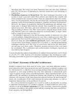
in the BSP model consists of a sequence of supersteps, see Fig. 4.8 for an illus-
tration. In each superstep, each component performs local computations and can
participate in point-to-point message transmissions. A local computation can be
performed in one time unit. The effect of message transmissions becomes visible

in the next time step, i.e., a receiver of a message can use the received data not
before the next superstep. At the end of each superstep, a barrier synchronization
is performed. There is a periodicity parameter L which determines the length of the
supersteps in time units. Thus, L determines the granularity of the computations.
The BSP model allows that the value of L can be controlled by the program to be
executed, even at runtime. There may be a lower bound for L given by the hardware.
The parallel program to be executed should set an upper bound for L such that in
each superstep, computations with approximately L steps can be assigned to each
processor.
190 4 Performance Analysis of Parallel Programs
barrier synchronization
barrier synchronization
time
superstep
local computations
global communication
virtual processors
Fig. 4.8 In the BSP model, computations are performed in supersteps where each superstep con-
sists of three phases: (1) simultaneous local computations of each processor, (2) communication
operations for data exchange between processors, and (3) a barrier synchronization to terminate
the communication operations and to make the data sent visible to the receiving processors. The
communication pattern shown for the communication phase represents an h-relation with h = 3
In each superstep, the router can implement arbitrary h-relations capturing com-
munication patterns, where each processor sends or receives at most h messages. A
computation in the BSP model can be characterized by four parameters [89]:
• p: the number of (virtual) processors used within the supersteps to perform com-
putations;
• s: the execution speed of the processors expressed as the number of computation
steps per seconds that each processor can perform, where each computation step
performs an (arithmetic or logical) operation on a local data element;

• l: the number of steps required for the execution of a barrier synchronization;
• g: the number of steps required on the average for the transfer of a memory word
in the context of an h-relation.
The parameter g is determined such that the execution of an h-relation with m
words per message takes l · m · g steps. For a real parallel computer, the value of
g depends not only on the bisection bandwidth of the interconnection network, see
p. 30, but also on the communication protocol used and on the implementation of
the communication library. The value of l is influenced not only by the diameter of
the interconnection network, but also by the implementation of the communication
library. Both l and g can be determined by suitable benchmark programs. Only p,l,
and g are independent parameters; the value of s is used for the normalization of the
values of l and g.
The execution time of a BSP program is specified as the sum of the execution
times of the supersteps which are performed for executing the program. The exe-
cution time T
superstep
of a single superstep consists of three terms: (1) the maximum
of the execution time w
i
for performing local computations of processor P
i
,(2)the
4.5 Parallel Computational Models 191
time for global communication for the implementation of an h-relation, and (3) the
time for the barrier synchronization at the end of each superstep. This results in
T
superstep
= max
processors
w

i
+h ·g +l.
The BSP model is a general model that can be used as a basis for different
programming models. To support the development of efficient parallel programs
with the BSP model, the BSPLib library has been developed [74, 89], which pro-
vides operations for the initialization of a superstep, for performing communication
operations, and for participating in the barrier synchronization at the end of each
superstep.
The BSP model has been extended to the Multi-BSP model, which extends the
original BSP model to capture important characteristics of modern architectures, in
particular multicore architectures [172]. In particular, the model is extended to a
hierarchical model with an arbitrary number d of levels modeling multiple memory
and cache levels. Moreover, at each level the memory size is incorporated as an addi-
tional parameter. The entire model is based on a tree of depth d with memory/caches
at the internal nodes and processors at the leaves.
4.5.3 LogP Model
In [34], several concerns about the BSP model are formulated. First, the length
of the supersteps must be sufficiently large to accommodate arbitrary h-relations.
This has the effect that the granularity cannot be decreased below a certain value.
Second, messages sent within a superstep can only be used in the next superstep,
even if the interconnection network is fast enough to deliver messages within the
same superstep. Third, the BSP model expects hardware support for synchronization
at the end of each superstep. Such support may not be available for some parallel
machines. Because of these concerns, the BSP model has been extended to the LogP
model to provide a more realistic modeling of real parallel machines.
Similar to the BSP model, the LogP model is based on the assumption that a
parallel computer consists of a set of processors with local memory that can com-
municate by exchanging point-to-point messages over an interconnection network.
Thus, the LogP model is also intended for the modeling of parallel computers
with a distributed memory. The communication behavior of a parallel computer is

described by four parameters:
• L (latency) is an upper bound on the latency of the network capturing the delay
observed when transmitting a small message over the network;
• o (overhead) is the management overhead that a processor needs for sending
or receiving a message; during this time, a processor cannot perform any other
operation;
• g (gap) is the minimum time interval between consecutive send or receive oper-
ations of a processor;
• P (processors) is the number of processors of the parallel machine.