13 Operation Scheduling: Algorithms and Applications 249
are needed. It is not clear as to which solution is better. Nor is it clear on the order
that we should perform scheduling and allocation.
Obviously, one possible method of design space exploration is to vary the con-
straints to probe for solutions in a point-by-point manner. For instance, you can
use some time constrained algorithm iteratively, where each iteration has a different
input latency. This will give you a number of solutions, and their various resource
allocations over a set of time points. Or you can run some resource constrained
algorithm iteratively. This will give you a latency for each of these area constraints.
Design space exploration problem has been the focus in numerous studies.
Though it is possible to formulate the problems using Integer Linear Program (ILP),
they quickly become intractable when the problem sizes get large. Much research
has been done to cleverly use heuristic approaches to address these problems. Actu-
ally, one major motivation of the popularly used Force Directed Scheduling (FDS)
algorithm [34] was to address the design space exploration task, i.e., by performing
FDS to solve a series timing constrained scheduling problems. In the same paper,
the authors also proposed a method called force-directed list scheduling (FDLS) to
address the resource constrained scheduling problem. The FDS method is construc-
tive since the solution is computed without backtracking. Every decision is made
deterministically in a greedy manner. If there are two potential assignments with the
same cost, the FDS algorithm cannot accurately estimate the best choice. Moreover,
FDS does not take into account future assignments of operators to the same control
step. Consequently, it is possible that the resulting solution will not be optimal due to
it’s greedy nature. FDS works well on small sized problems, however, it often results
to inferior solutions for more complex problems. This phenomena is observed in our
experiments reported in Sect. 13.4.
In [16], the authors concentrate on providing alternative “module bags” for
design space exploration by heuristically solving the clique partitioning problems
and using force directed scheduling. Their work focuses more on the situations
where the operations in the design can be executed on alternative resources. In the
Voyager system [11], scheduling problems are solved by carefully bounding the

design space using ILP, and good results are reported on small sized benchmarks.
Moreover, it reveals that clock selection can have an important impact on the final
performance of the application. In [14,21,32], genetic algorithms are implemented
for design space exploration. Simulated annealing [29] has also been applied in this
domain. A survey on design space exploration methodologies can be found in [28]
and [9].
In this chapter, we focus our attention on the basic design space exploration prob-
lem similar to the one treated in [34], where the designers are faced with the task
of mapping a well defined application represented as a DFG onto a set of known
resources where the compatibility between the operations and the resource types has
been defined. Furthermore, the clock selection has been determined in the form of
execution cycles for the operations. The goal is to find the a Pareto optimal tradeoff
amongst the design implementations with regard to timing and resource costs. Our
basic method can be extended to handle clock selection and the use of alternative
resources. However, this is beyond the scope of this discussion.
250 G. Wang et al.
13.5.2 Exploration Using Time and Resource Constrained Duality
As we have discussed, traditional approaches solve the design space exploration task
solving a series of scheduling problems, using either a resource constrained method
or a timing constrained method. Unfortunately, designers are left with individual
tools for tackling either problem. They are faced with questions like: Where do we
start the design space exploration? What is the best way to utilize the scheduling
tools? When do we stop the exploration?
Moreover, due to the lack of connection amongst the traditional methods, there
is very little information shared between time constrained and resource constrained
solutions. This is unfortunate, as we are throwing away potential solutions since
solving one problem can offer more insight into the other problem. Here we pro-
pose a novel design exploration method that exploits the duality of the time and
resource constrained scheduling problems. Our exploration automatically constructs
a time/area tradeoff curve in a fast, effective manner. It is a general approach and

can be combined with any high quality scheduling algorithm.
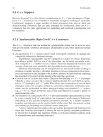
We are concerned with the design problem of making tradeoffs between hardware
cost and timing performance. This is still a commonly faced problem in practice, and
other system metrics, such as power consumption, are closely related with them.
Based on this, we have a 2-D design space as illustrated in Fig. 13.1a, where the x-
axis is the execution deadline and the y-axis is the aggregated hardware cost. Each
point represents a specific tradeoff of the two parameters.
For a given application, the designer is given R types of computing resources
(e.g., multipliers and adders) to map the application to the target device. We define
a specific design as a configuration, which is simply the number of each specific
resource type. In order to keep the discussion simple, in the rest of the paper we
14 16 18 20 22 24 26 28 30
deadline (cycle)
50
100
150
200
250
300
350
cost
design space
L
c
1
t
1
t
2
(m

1
,a
1
)(m
2
,a
2
)
F
U
deadline (cycle)
cost
design space
L
TCSTCSTCS
RCS
RCS
(m
1
,a
1
)
(m
2
,a
2
)
(m
3
,a

3
)
(m?,a?)
t
1
t
2
-1t
3
-1 t
2
t
3
F
U
(a) (b)
Fig. 13.1 Design space exploration using duality between schedule problems (curve L gives the
optimal time/cost tradeoffs)
13 Operation Scheduling: Algorithms and Applications 251
assume there are only two resource types M (multiply) and A (add), though our
algorithm is not limited to this constraint. Thus, each configuration can be specified
by (m,a) where m is the number of resource M and a is the number of A. For each
specific configuration we have the following lemma about the portion of the design
space that it maps to.
Lemma 1. Let C be a feasible configuration with cost c for the target application.
The configuration maps to a horizontal line in the design space starting at (t
min
,c),
where t
min

is the resource constrained minimum scheduling time.
The proof of the lemma is straightforward as each feasible configuration has a
minimum execution time t
min
for the application, and obviously it can handle every
deadline longer than t
min
. For example, in Fig. 13.1a, if the configuration (m
1
,a
1
)
has a cost c
1
and a minimum scheduling time t
1
, the portion of design space that
it maps to is indicated by the arrow next to it. Of course, it is possible for another
configuration (m
2
,a
2
) to have the same cost but a bigger minimum scheduling time
t
2
. In this case, their feasible space overlaps beyond (t
2
,c
1
).

As we discussed before, the goal of design space exploration is to help the
designer find the optimal tradeoff between the time and area. Theoretically, this
can be done by finding the minimum area c amongst all the configurations that are
capable of producing t ∈ [t
asap
,t
seq
],wheret
asap
is the ASAP time for the applica-
tion while t
seq
is the sequential execution time. In other words, we can find these
points by performing time constrained scheduling (TCS) on all t in the interested
range. These points form a curve in the design space, as illustrated by curve L in
Fig. 13.1a. This curve divides the design space into two parts, labeled with F and U
respectively in Fig. 13.1a, where all the points in F are feasible to the given applica-
tion while U contains all the unfeasible time/area pairs. More interestingly, we have
the following attribute for curve L:
Lemma 2. Curve L is monotonically non-increasing as the deadline t increases.
1
Due to this lemma, we can use the dual solution of finding the tradeoff curve by
identifying the minimum resource constrained scheduling (RCS) time t amongst all
the configurations with cost c. Moreover, because the monotonically non-increasing
property of curve L, there may exist horizontal segments along the curve. Based
on our experience, horizontal segments appear frequently in practice. This moti-
vates us to look into potential methods to exploit the duality between RCS and TCS
to enhance the design space exploration process. First, we consider the following
theorem:
Theorem 1. If C is a configuration that provides the minimum cost at time t

1
,then
the resource constrained scheduling result t
2
of C satisfies t
2
 t
1
. More importantly,
there is no configuration C

with a smaller cost that can produce an execution time
within [t
2
,t
1
].
2
1
Proof is omitted because of page limitation.
2
Proof is omitted because of page limitation.
252 G. Wang et al.
This theorem provides a key insight for the design space exploration problem. It
says that if we can find a configuration with optimal cost c at time t
1
, we can move
along the horizontal segment from (t
1
,c) to (t

2
,c) without losing optimality. Here
t
2
is the RCS solution for the found configuration. This enables us to efficiently
construct the curve L by iteratively using TCS and RCS algorithms and leveraging
the fact that such horizontal segments do frequently occur in practice. Based on
the above discussion, we propose a new space exploration algorithm as shown in
Algorithm 1 that exploits the duality between RCS and TCS solutions. Notice the
min function in step 10 is necessary since a heuristic RCS algorithm may not return
the true optimal that could be worse than t
cur
.
By iteratively using the RCS and TCS algorithms, we can quickly explore the
design space. Our algorithm provides benefits in runtime and solution quality com-
pared with using RCS or TCS alone. Our algorithm performs exploration starting
from the largest deadline t
max
. Under this case, the TCS result will provide a con-
figuration with a small number of resources. RCS algorithms have a better chance
to find the optimal solution when the resource number is small, therefore it pro-
vides a better opportunity to make large horizontal jumps. On the other hand, TCS
algorithms take more time and provide poor solutions when the deadline is uncon-
strained. We can gain significant runtime savings by trading off between the RCS
and TCS formulations.
The proposed framework is general and can be combined with any scheduling
algorithm. We found that in order for it to work in practice, the TCS and RCS
algorithms used in the process require special characteristics. First, they must be
fast, which is generally requested for any design space exploration tool. More
importantly, they must provide close to optimal solutions, especially for the TCS

problem. Otherwise, the conditions for Theorem 1 will not be satisfied and the gen-
erated curve L will suffer significantly in quality. Moreover, notice that we enjoy the
biggest jumps when we take the minimum RCS result amongst all the configurations
Algorithm 1 Iterative design space exploration algorithm
procedure DSE
output:curveL
1: interested time range [t
min
,t
max
],wheret
min
 t
asap
and t
max
 t
seq
.
2: L =
φ
3: t
cur
= t
max
4: while t
cur
 t
min
do

5: perform TCS on t
cur
to obtain the optimal configurations C
i
.
6: for configuration C
i
do
7: perform RCS to obtain the minimum time t
i
rcs
8: end for
9: t
rcs
= min
i
(t
i
rcs
) /* find the best rcs time */
10: t
cur
= min(t
cur
,t
rcs
) −1
11: extend L based on TCS and RCS results
12: end while
13: return L

13 Operation Scheduling: Algorithms and Applications 253
that provide the minimum cost for the TCS problem. This is reflected in Steps 6–9
in Algorithm 1. For example, it is possible that both (m,a) and (m

,a

) provide the
minimum cost at time t but they have different deadline limits. Therefore a good
TCS algorithm used in the proposed approach should be able to provide multiple
candidate solutions with the same minimum cost, if not all of them.
13.6 Conclusion
In this chapter, we provide a comprehensive survey on various operation schedul-
ing algorithms, including List Scheduling, Force-Directed Scheduling, Simulated
Annealing, Ant Colony Optimization (ACO) approach, together with others. We
report our evaluation for the aforementioned algorithms against a comprehensive set
of benchmarks,called ExpressDFG. We give the characteristics of these benchmarks
and discuss suitability for evaluating scheduling algorithms. We present detailed
performance evaluation results in regards of solution quality, stability of the algo-
rithms, their scalability over different applications and their runtime efficiency. As
a direct application, we present a uniformed design space exploration method that
exploits duality between the timing and resource constrained scheduling problems.
Acknowledgment This work was partially supported by National Science Foundation Grant
CNS-0524771.
References
1. Aarts, E. and Korst, J. (1989). Simulated Annealing and Boltzmann Machines: A Stochastic
Approach to Combinatorial Optimization and Neural Computing. Wiley, New York, NY.
2. Adam, T. L., Chandy, K. M., and Dickson, J. R. (1974). A comparison of list schedules for
parallel processing systems. Communications of the ACM, 17(12):685–690.
3. Aigner, G., Diwan, A., Heine, D. L., Moore, M. S. L. D. L., Murphy, B. R., and Sapuntzakis,
C. (2000). The Basic SUIF Programming Guide. Computer Systems Laboratory, Stanford

University.
4. Alet`a, A., Codina, J. M., and and Antonio G., Jes´us S. (2001). Graph-Partitioning Based
Instruction Scheduling for ClusteredProcessors. In Proceedings of the 34th Annual ACM/IEEE
International Symposium on Microarchitecture.
5. Auyeung, A., Gondra, I., and Dai, H. K. (2003). Integrating random ordering into multi-
heuristic list scheduling genetic algorithm. Advances in Soft Computing: Intelligent Systems
Design and Applications. Springer, Berlin Heidelberg New York.
6. Beaty, Steve J. (1993). Genetic algorithms versus tabu search for instruction scheduling.
In Proceedings of the International Conference on Artificial Neural Networks and Genetic
Algorithms.
7. Beaty, Steven J. (1991). Genetic algorithms and instruction scheduling. In Proceedings of the
24th Annual International Symposium on Microarchitecture.
8. Bernstein, D., Rodeh, M., and Gertner, I. (1989). On the Complexity of Scheduling Problems
for Parallel/PipelinedMachines. IEEE Transactions on Computers, 38(9):1308–1313.
254 G. Wang et al.
9. C. McFarland, M., Parker, A. C., and Camposano, R. (1990). The high-level synthesis of
digital systems. In Proceedings of the IEEE, vol. 78, pp. 301–318.
10. Camposano, R. (1991). Path-based scheduling for synthesis. IEEE Transaction on Computer-
Aided Design, 10(1):85–93.
11. Chaudhuri, S., Blythe, S. A., and Walker, R. A. (1997). A solution methodology for exact
design space exploration in a three-dimensional design space. IEEE Transactions on very
Large Scale Integratioin Systems, 5(1):69–81.
12. Corne, D., Dorigo, M., and Glover, F., editors (1999). New Ideas in Optimization.McGraw
Hill, London.
13. Deneubourg, J. L. and Goss, S. (1989). Collective Patterns and Decision Making. Ethology,
Ecology and Evolution, 1:295–311.
14. Dick, R. P. and Jha, N. K. (1997). MOGAC: A Multiobjective Genetic Algorithm for the Co-
Synthesis of Hardware-Software Embedded Systems. In IEEE/ACM Conference on Computer
Aided Design, pp. 522–529.
15. Dorigo, M., Maniezzo, V., and Colorni, A. (1996). Ant System: Optimization by a Colony

of Cooperating Agents. IEEE Transactions on Systems, Man and Cybernetics, Part-B,
26(1):29–41.
16. Dutta, R., Roy, J., and Vemuri, R. (1992). Distributed design-space exploration for high-level
synthesis systems. In DAC ’92, pp. 644–650. IEEE Computer Society Press, Los Alamitos,
CA.
17. ExpressDFG (2006). ExpressDFG benchmark web site. />benchmark/.
18. Grajcar, M. (1999). Genetic List Scheduling Algorithm for Scheduling and Allocationon
a Loosely Coupled Heterogeneous Multiprocessor System. In Proceedings of the 36th
ACM/IEEE Conference on Design Automation Conference.
19. Gutjahr, W. J. (2002). Aco algorithms with guaranteed convergence to the optimal solution.
Information Processing Letters, 82(3):145–153.
20. Heijligers, M. and Jess, J. (1995). High-level synthesis scheduling and allocation using
genetic algorithms based on constructive topological scheduling techniques. In International
Conference on Evolutionary Computation, pp. 56–61, Perth, Australia.
21. Heijligers, M. J. M., Cluitmans, L. J. M., and Jess, J. A. G. (1995). High-level synthesis
scheduling and allocation using genetic algorithms. p. 11.
22. Hu, T. C. (1961). Parallel sequencing and assembly line problems. Operations Research,
9(6):841–848.
23. Kennedy, K. and Allen, R. (2001). Optimizing Compilers for Modern Architectures: A
Dependence-basedApproach. Morgan Kaufmann, San Francisco.
24. Kernighan, B. W. and Lin, S. (1970). An efficient heuristic procedure for partitioning graphs.
Bell System Technical Journal, 49(2):291–307.
25. Kolisch, R. and Hartmann, S. (1999). Heuristic algorithms for solving the resource-
constrained project scheduling problem: classification and computational analysis. Project
Scheduling: Recent Models, Algorithms and Applications. Kluwer Academic, Dordrecht.
26. Lee, C., Potkonjak, M., and Mangione-Smith, W. H. (1997). Mediabench: A tool for evaluating
and synthesizing multimedia and communications systems. In Proceedings of the 30th Annual
ACM/IEEE International Symposium on Microarchitecture.
27. Lee, J H., Hsu, Y C., and Lin, Y L. (1989). A new integer linear programming formulation
for the scheduling problem in data path synthesis. In Proceedings of ICCAD-89, pp. 20–23,

Santa Clara, CA.
28. Lin, Y L. (1997). Recent developments in high-level synthesis. ACM Transactions on Design
of Automation of Electronic Systems, 2(1):2–21.
29. Madsen, J., Grode, J., Knudsen, P. V., Petersen, M. E., and Haxthausen, A. (1997). LYCOS:
The Lyngby Co-Synthesis System. Design Automation for Embedded Systems, 2(2):125–63.
30. Memik, S. O., Bozorgzadeh, E., Kastner, R., and MajidSarrafzadeh (2001). A super-scheduler
for embedded reconfigurable systems. In IEEE/ACM International Conference on Computer-
Aided Design.
13 Operation Scheduling: Algorithms and Applications 255
31. Micheli, G. De (1994). Synthesis and Optimization of Digital Circuits. McGraw-Hill, New
Yo rk.
32. Palesi, M. and Givargis, T. (2002). Multi-Objective Design Space Exploration Using Genet-
icAlgorithms. In Proceedings of the Tenth International Symposium on Hardware/Software-
Codesign.
33. Park, I C. and Kyung, C M. (1991). Fast and near optimal scheduling in automatic data path
synthesis. In DAC ’91: Proceedings of the 28th conference on ACM/IEEE design automation,
pp. 680–685. ACM Press, New York, NY.
34. Paulin, P. G. and Knight, J. P. (1987). Force-directed scheduling in automatic data path
synthesis. In 24th ACM/IEEE Conference Proceedings on Design Automation Conference.
35. Paulin, P. G. and Knight, J. P. (1989). Force-directed scheduling for the behavioral synthesis
of asic’s. IEEE Transactions on Computer-Aided Design, 8:661–679.
36. Poplavko, P., van Eijk, C. A. J., and Basten, T. (2000). Constraint analysis and heuris-
tic scheduling methods. In Proceedings of 11th Workshop on Circuits, Systems and Signal
Processing(ProRISC2000), pp. 447–453.
37. Schutten, J. M. J. (1996). List scheduling revisited. Operation Research Letter, 18:167–170.
38. Semiconductor Industry Association (2003). National Technology Roadmap for Semiconduc-
tors.
39. Sharma, A. and Jain, R. (1993). Insyn: Integrated scheduling for dsp applications. In DAC, pp.
349–354.
40. Smith, J. E. (1989). Dynamic instruction scheduling and the astronautics ZS-1. IEEE

Computer, 22(7):21–35.
41. Smith, M. D. and Holloway, G. (2002). An Introduction to Machine SUIF and Its Portable
Librariesfor Analysis and Optimization. Division of Engineering and Applied Sciences,
Harvard University.
42. St¨utzle, T. and Hoos, H. H. (2000). MAX–MIN Ant System. Future Generation Computer
Systems, 16(9):889–914.
43. Sweany, P. H. and Beaty, S. J. (1998). Instruction scheduling using simulated annealing. In
Proceedings of 3rd International Conference on Massively Parallel Computing Systems.
44. Topcuouglu, H., Hariri, S., and you Wu, M. (2002). Performance-effective and low-complexity
task scheduling for heterogeneous computing. IEEE Transactions on Parallel and Distributed
Systems, 13(3):260–274.
45. Verhaegh, W. F. J., Aarts, E. H. L., Korst, J. H. M., and Lippens, P. E. R. (1991). Improved
force-directed scheduling. In EURO-DAC ’91: Proceedings of the Conference on European
Design Automation, pp. 430–435. IEEE Computer Society Press, Los Alamitos, CA.
46. Verhaegh, W. F. J., Lippens, P. E. R., Aarts, E. H. L., Korst, J. H. M., van der Werf, A.,
and van Meerbergen, J. L. (1992). Efficiency improvements for force-directed scheduling.
In ICCAD ’92: Proceedings of the 1992 IEEE/ACM international Conference on Computer-
Aided Design, pp. 286–291. IEEE Computer Society Press, Los Alamitos, CA.
47. Wang, G., Gong, W., DeRenzi, B., and Kastner, R. (2006). Ant Scheduling Algorithms for
Resource and Timing Constrained Operation Scheduling. IEEE Transactions of Computer-
Aided Design of Integrated Circuits and Systems (TCAD), 26(6):1010–1029.
48. Wang, G., Gong, W., and Kastner, R. (2003). A New Approach for Task Level Computa-
tional ResourceBi-partitioning. 15th International Conference on Parallel and Distributed
Computing and Systems, 1(1):439–444.
49. Wang, G., Gong, W., and Kastner, R. (2004). System level partitioning for programmable plat-
forms using the ant colony optimization. 13th International Workshop on Logic and Synthesis,
IWLS’04.
50. Wang, G., Gong, W., and Kastner, R. (2005). Instruction scheduling using MAX–MIN ant
optimization. In 15th ACM Great Lakes Symposium on VLSI, GLSVLSI’2005.
51. Wiangtong, T., Cheung, P. Y. K., and Luk, W. (2002). Comparing Three Heuristic Search

Methods for FunctionalPartitioning in Hardware-Software Codesign. Design Automation for
Embedded Systems, 6(4):425–49.
Chapter 14
Exploiting Bit-Level Design Techniques
in Behavioural Synthesis
Mar´ıa Carmen Molina, Rafael Ruiz-Sautua, Jos´e Manuel Mend´ıas,
and Rom´an Hermida
Abstract Most conventional high-level synthesis algorithms and commercial tools
handle specification operations in a very conservative way, as they assign opera-
tions to one or several consecutive clock cycles, and to one functional unit of equal
or larger width. Independently of the parameter to be optimized, area, execution
time, or power consumption, more efficient implementations could be derived from
handling operations at the bit level. This way, one operation can be decomposed
into several smaller ones that may be executed in several inconsecutive cycles and
over several functional units. Furthermore, the execution of one operation fragment
can begin once its input operands are available, even if the calculus of its pre-
decessors finishes at a later cycle, and also arithmetic properties can be partially
applied to specification operations. These design strategies may be either exploited
within the high-level synthesis, or applied to optimize behavioural specifications or
register-transfer-level implementations.
Keywords: Scheduling, Allocation, Binding, Bit-level design
14.1 Introduction
Conventional High-Level Synthesis (HLS) algorithms and commercial tools derive
Register-Transfer-Level (RTL) implementations from behavioural specifications
subject to some constraints in terms of area, execution time, or power consump-
tion. Most algorithms handle specification operations in a very conservative way. In
order to reduce one or more of the already mentioned parameters, they assign oper-
ations to one or several consecutive clock cycles, and to one functional unit (FU) of
equal or larger width. These bindings represent quite a limited subset of all possible
ones, whose consideration would surely lead to better designs.

If circuit area becomes the parameter to be minimized, then conventional HLS
algorithms usually try to balance the number of operations executed per cycle, as
P. Coussy and A. Morawiec (eds.) High-Level Synthesis.
c
 Springer Science + Business Media B.V. 2008
257
258 M.C. Molina et al.
well as keep HW resources busy in most cycles. Since a perfect distribution of oper-
ations among cycles is nearly impossible to be reached, some HW waste (idle HW
resources) appears in almost every cycle. This waste is mainly due to the following
two factors: operation mobility (range of cycles in which every operation may start
its execution, subject to data dependencies and given timing constraints), and speci-
fication heterogeneity (in function of the number of different types, widths, and data
formats present in the behavioural specification).
Operation mobility influences the HW waste because a limited mobility makes
perfect distributions of operations among cycles unreachable. Even in the hypothet-
ical case of specifications without data dependencies, some waste appears as long
as the latency is not a divisor of the number of operations.
Specification heterogeneity influences the HW waste because HLS algorithms
usually treat separately operations with different types, data formats or widths, pre-
venting them from sharing the same HW resource. In consequence, a particular
mobility dependent waste emerges for every different (type, data format, width)
triplet in the specification. This waste exists even if more efficient HLS algorithms
are used. For example, many algorithms are able to allocate operations of different
widths to the same FU. But if an operation is executed over a wider FU (extending
its arguments) it is partially wasted. Besides, in most cases, the cycle length is longer
than necessary because the most significant bits (MSB) of the calculated results are
discarded. The HW waste also arises in implementations with arithmetic-logic units
(ALU) able to execute different types of operations. In this case, part of the ALU
always remains unused while it executes any operation.

On one hand, the mobility dependent waste could be reduced through the balance
in the number of bits of every different operation type calculated per cycle, instead
of the number of operations. In order to obtain homogeneous distributions, some
specification operations should be transformed into a set of new ones, whose types
and widths might be different from the original. On the other hand, the heterogeneity
dependent waste could be reduced if all compatible operations were synthesized
jointly (two operations are compatible if they can be executed over same type FUs
and some glue logic). To do so, algorithms able to fragment compatible operations
into their common operative kernel plus some glue logic are needed.
In both cases, each operation fragment inherits the mobility of the original opera-
tion and is scheduled separately. Therefore, one original operation may be executed
across a set of cycles, not necessarily consecutive (saving the partial results and
carry outs calculated in every cycle), and bound to a set of linked HW resources
in each cycle. It might occur that the first operation fragment executed is not the
one that uses the least significant bits (LSB) of the input operands, although this
feature does not imply that the MSB of the result can be calculated before its LSB.
In the datapaths designed following these strategies the number, type, and width of
the HW resources are, in general, independent of the number, type, and width of the
specification operations and variables.
The example in Fig. 14.1 illustrates the main features of these design strate-
gies. It shows a fragment of a data flow graph obtained from a multiple precision
specification with multiplications and additions, and two schedules proposed by
14 Exploiting Bit-Level Design Techniques in Behavioural Synthesis 259
Fig. 14.1 DFG of a behavioural specification, conventional schedule, and more efficient schedule
based on operation fragmentations
a conventional algorithm and by a HLS algorithm including some fragmentation
techniques. While every operation is executed in a single cycle in the conventional
schedule, some operations are executed during several cycles in the second one.
However, this feature should not be confused with multi cycle operators. The main
advantages of this new design method follow below: one operation can be sched-

uled in several non consecutive cycles, different FUs can be used to compute every
operation fragment, the FUs needed to execute every fragment are narrower than
the original operation, and the storage of all the input operand bits is not needed all
the time the operation is being executed. In the example, the addition R = P+ Q is
scheduled in the first and second cycles, and the multiplication N = L ×M in the
first and third cycles. In this case, the set of cycles selected to execute N = L ×M
are not consecutive. Note also that the multiplication fragment scheduled in the first
cycle (L ×M
11 8
) is not the one that calculates the LSB of the original operation.
Table 14.1 shows the set of cycles and FUs selected to execute every specification
operation. Operations I = H ×G, N = L×M,andR = P+ Q have been fragmented
into several new operations as shown in the table. In order to balance the computa-
tional cost of the operations executed per cycle, N = L×M and R = P+Q have been
fragmented by the proposed scheduling algorithm into seven and two new opera-
tions, respectively. And in order to minimize the FUs area (increasing FUs reuse),
I = H ×G has been fragmented into five new operations, which are then executed
over three multipliers and two adders. Figure 14.2 illustrates how the execution of
N = L ×M, that begins in the first cycle, is completed in the third one over three
multipliers and three adders.