13 Operation Scheduling: Algorithms and Applications 239
One of the first problems to which ACO was successfully applied was the Travel-
ing Salesman Problem (TSP) [15], for which it gave competitive results comparing
with traditional methods. Researchers have since formulated ACO methods for a
variety of traditional NP-hard problems. These problems include the maximum
clique problem, the quadratic assignment problem, the graph coloring problem,
the shortest common super-sequence problem, and the multiple knapsack problem.
ACO also has been applied to practical problems such as the vehicle routing prob-
lem, data mining, network routing problem and the system level task partitioning
problem [12, 48,49].
It was shown [19] that ACO converges to an optimal solution with probability
of exactly one; however there is no constructive way to guarantee this. Balancing
exploration to achieve close-to-optimal results within manageable time remains an
active research topic for ACO algorithms. MAX–MIN Ant System (MMAS) [42] is
a popularly used method to address this problem. MMAS is built upon the original
ACO algorithm, which improves it by providing dynamically evolving bounds on
the pheromone trails so that the heuristic never strays too far away from the best
encountered solution. As a result, all possible paths will have a non-trivial prob-
ability of being selected; thus it encourages broader exploration of the search
space while maintaining a good differential between alternative solutions. It was
reported that MMAS was the best performing ACO approach on a number of classic
combinatory optimization tasks.
Both time constrained and resource constrained scheduling problems can be
effectively solved by using ACO. Unfortunately, in the consideration of space, we
can only give a general introduction on the ACO formulation for the TCS prob-
lem. For a complete treatment of the algorithms, including detailed discussion on
the algorithms’ implementation, applicability, complexity, extensibility, parameter
selection and performance, please refer to [47, 50].
In its ACO-based formulation, the TCS problem is solved with an iterative
searching process. the algorithms employ a collection of agents that collaboratively
explore the search space. A stochastic decision making strategy is applied in order

to combine global and local heuristics to effectively conduct this exploration. As
the algorithm proceeds in finding better quality solutions, dynamically computed
local heuristics are utilized to better guide the searching process. Each iteration
consists of two stages. First, the ACO algorithm is applied where a collection of
ants traverse the DFG to construct individual operation schedules with respect to
the specified deadline using global and local heuristics. Secondly, these scheduling
results are evaluated using their resource costs. The associated heuristics are then
adjusted based on the solutions found in the current iteration. The hope is that future
iterations will benefit from this adjustment and come up with better schedules.
Each operation or DFG node op
i
is associated with D pheromone trails
τ
ij
,where
j = 1, ,D and D is the specified deadline. These pheromone trails indicate the
global favorableness of assigning the ith operation at the jth control step in order
to minimize the resource cost with respect to the time constraint. Initially, based on
ASAP and ALAP results,
τ
ij
is set with some fixed value
τ
0
if j is a valid control
step for op
i
;otherwise,itissettobe0.
240 G. Wang et al.
For each iteration, m ants are released and each ant individually starts to con-

struct a schedule by picking an unscheduled instruction and determining its desired
control step. However, unlike the deterministic approach used in the FDS method,
each ant picks up the next instruction for scheduling decision probabilistically. Once
an instruction op
h
is selected, the ant needs to make decision on which control
step it should be assigned. This decision is also made probabilistically as illustrated
in (13.6).
p
hj
=
⎧
⎨
⎩
τ
hj
(t)
α
·
η
β
hj
∑
l
(
τ
α
hl
(t)·
η

β
hl
)
if op
h
can be scheduled at l and j
0otherwise
(13.6)
Here j is the time step under consideration. The item
η
hj
is the local heuristic for
scheduling operation op
h
at control step j,and
α
and
β
are parameters to control
the relative influence of the distributed global heuristic
τ
hj
and local heuristic
η
hj
.
Assuming op
h
is of type k,
η

hj
to simply set to be the inverse of the distribution
graph value [34], which is computed based on partial scheduling result and is an
indication on the number of computing units of type k needed at control step j.In
other words, an ant is more likely to make a decision that is globally considered
“good” and also uses the fewest number of resources under the current partially
scheduled result. We do not recursively compute the forces on the successor nodes
and predecessor nodes. Thus, selection is much faster. Furthermore, the time frames
are updated to reflect the changed partial schedule. This guarantees that each ant
will always construct a valid schedule.
In the second stage of our algorithm, the ant’s solutions are evaluated. The quality
of the solution from ant h is judged by the total number of resources, i.e., Q
h
=
∑
k
r
k
.
At the end of the iteration, the pheromone trail is updated according to the quality
of individual schedules. Additionally, a certain amount of pheromone evaporates.
More specifically, we have:
τ
ij
(t)=
ρ
·
τ
ij
(t)+

m
∑
h=1
Δτ
h
ij
(t) where 0 <
ρ
< 1. (13.7)
Here
ρ
is the evaporation ratio, and
Δτ
h
ij
=

Q/Q
h
if op
i
is scheduled at j by ant h
0otherwise
(13.8)
Q is a fixed constant to control the delivery rate of the pheromone. Two important
operations are performed in the pheromone trail updating process. Evaporation is
necessary for ACO to effectively explore the solution space, while reinforcement
ensures that the favorable operation orderings receive a higher volume of pheromone
and will have a better chance of being selected in the future iterations. The above
process is repeated multiple times until an ending condition is reached. The best

result found by the algorithm is reported.
13 Operation Scheduling: Algorithms and Applications 241
Comparing with the FDS method, the ACO algorithm differs in several aspects.
First, rather than using a one-time constructive approach based on greedy local deci-
sions, the ACO method solves the problem in an evolutionary manner. By using
simple local heuristics, it allows individual scheduling result to be generated in a
faster manner. With a collection of such individual results and by embedding and
adjusting global heuristics associated with partial solutions, it tries to learn during
the searching process. By adopting a stochastic decision making strategy consid-
ering both global experience and local heuristics, it tries to balance the efforts of
exploration and exploitation in this process. Furthermore, it applies positive feed-
back to strengthen the “good” partial solutions in order to speed up the convergence.
Of course, the negative effect is that it may fall into local minima, thus requires com-
pensation measures such as the one introduced in MMAS. In our experiments, we
implemented both the basic ACO and the MMAS algorithms. The latter consistently
achieves better scheduling results, especially for larger DFGs.
13.4 Performance Evaluation
13.4.1 Benchmarks and Setup
In order to test and evaluate our algorithms, we have constructed a comprehen-
sive set of benchmarks named ExpressDFG. These benchmarks are taken from one
of two sources: (1) popular benchmarks used in previous literature; (2) real-life
examples generated and selected from the MediaBench suite [26].
The benefit of having classic samples is that they provide a direct comparison
between results generated by our algorithm and results from previously published
methods. This is especially helpful when some of the benchmarks have known opti-
mal solutions. In our final testing benchmark set, seven samples widely used in
instruction scheduling studies are included. These samples focus mainly on fre-
quently used numeric calculations performed by different applications. However,
these samples are typically small to medium in size, and are considered somewhat
old. To be representative, it is necessary to create a more comprehensive set with

benchmarks of different sizes and complexities. Such benchmarks shall aim to:
– Provide real-life testing cases from real-life applications
– Provide more up-to-date testing cases from modern applications
– Provide challenging samples for instruction scheduling algorithms with regards
to larger number of operations, higher level of parallelism and data dependency
– Provide a wide range of synthesis problems to test the algorithms’ scalability
For this purpose, we investigated the MediaBench suite, which contains a wide
range of complete applications for image processing, communications and DSP
applications. We analyzed these applications using the SUIF [3] and Machine SUIF
[41] tools, and over 14,000 DFGs were extracted as preliminary candidates for our
242 G. Wang et al.
Table 13.1 ExpressDFG benchmark suite
Benchmark name No. nodes No. edges ID
HAL 11 8 4
horner
bezier
†
18 16 8
ARF 28 30 8
motion
vectors
†
32 29 6
EWF 34 47 14
FIR2 40 39 11
FIR1 44 43 11
h2v2
smooth downsample
†
51 52 16

feedback
points
†
53 50 7
collapse
pyr
†
56 73 7
COSINE1 66 76 8
COSINE2 82 91 8
write
bmp header
†
106 88 7
interpolate
aux
†
108 104 8
matmul
†
109 116 9
idctcol 114 164 16
jpeg
idct ifast
†
122 162 14
jpeg
fdct islow
†
134 169 13

smooth
color z triangle
†
197 196 11
invert
matrix general
†
333 354 11
Benchmarks with † are extracted from MediaBench
benchmark set. After careful study, thirteen DFG samples were selected from four
MediaBench applications: JPEG, MPEG2, EPIC and MESA.
Table 13.1 lists all 20 benchmarks that were included in our final benchmark set.
Together with the names of the various functions where the basic blocks originated
are the number of nodes, number of edges and instruction depth (assuming unit
delay for every instruction) of the DFG. The data, including related statistics, DFG
graphs and source code for the all testing benchmarks, is available online [17].
For all testing benchmarks, operations are allocated on two types of computing
resources, namely MUL and ALU, where MUL is capable of handling multipli-
cation and division, and ALU is used for other operations such as addition and
subtraction. Furthermore, we define the operations running on MUL to take two
clock cycles and the ALU operations take one. This definitely is a simplified case
from reality. However, it is a close enough approximation and does not change
the generality of the results. Other choices can easily be implemented within our
framework.
13.4.2 Time Constrained Scheduling: ACO vs. FDS
With the assigned resource/operation mapping, ASAP is first performed to find the
critical path delay L
c
. We then set our predefined deadline range to be [L
c

,2L
c
], i.e.,
13 Operation Scheduling: Algorithms and Applications 243
from the critical path delay to two times of this delay. This results 263 testing cases
in total. For each delay, we run FDS first to obtain its scheduling result. Following
this, the ACO algorithm is executedfive times to obtain enough data for performance
evaluation. We report the FDS result quality, the average and best result quality for
the ACO algorithm and the standard deviation for these results. The execution time
information for both algorithms is also reported.
We have implemented the ACO formulation in C for the TCS problem. The evap-
oration rate
ρ
is configured to be 0.98. The scaling parameters for global and local
heuristics are set to be
α
=
β
= 1 and delivery rate Q = 1. These parameters are
not changed over the tests. We also experimented with different ant number m and
the allowed iteration count N. For example, set m to be proportional to the average
branching factor of the DFG under study and N to be proportional to the total oper-
ation number. However, it is found that there seems to exist a fixed value pair for m
and N which works well across the wide range of testing samples in our benchmark.
In our final settings, we set m to be 10, and N to be 150 for all the timing constrained
scheduling experiments.
Based on our experiments, the ACO based operation scheduling achieves bet-
ter or much better results. Our approach seems to have much stronger capability in
robustly finding better results for different testing cases. Furthermore, it scales very
well over different DFG sizes and complexities. Another aspect of scalability is the

pre-defined deadline. The average result quality generated by the ACO algorithm
is better than or equal to the FDS results in 258 out of 263 cases. Among them,
for 192 testing cases (or 73% of the cases) the ACO method outperforms the FDS
method. There are only five cases where the ACO approach has worse average qual-
ity results. They all happened on the invert
matrix general benchmark. On average,
we can expect a 16.4% performance improvement over FDS. If only considering the
best results among the five runs for each testing case, we achieve a 19.5% resource
reduction averaged over all tested samples. The most outstanding results provided
by the ACO method achieve a 75% resource reduction compared with FDS. These
results are obtained on a few deadlines for the jpeg
idct ifast benchmark.
Besides absolute quality of the results, one difference between FDS and the
ACO method is that ACO method is relatively more stable. In our experiments, it is
observed that the FDS approach can provide worse quality results as the deadline is
relaxed. Using the idctcol as an example, FDS provides drastically worse results for
deadlines ranging from 25 to 30 though it is able to reach decent scheduling qual-
ities for deadline from 19 to 24. The same problem occurs for deadlines between
36 and 38. One possible reason is that as the deadline is extended, the time frame
of each operation is also extended, which makes the force computation more likely
to clash with similar values. Due to the lack of backtracking and good look-ahead
capability, an early mistake would lead to inferior results. On the other hand, the
ACO algorithm robustly generates monotonically non-increasing results with fewer
resource requirements as the deadline increases.
244 G. Wang et al.
13.4.3 Resource Constrained Scheduling: ACO vs. List Scheduling
and ILP
We have implemented the ACO-based resource-constrained scheduling algorithm
and compared its performance with the popularly used list scheduling and force-
directed scheduling algorithms.

For each of the benchmark samples, we run the ACO algorithm with different
choices of local heuristics. For each choice, we also perform five runs to obtain
enough statistics for evaluating the stability of the algorithm. Again we fixed the
number of ants per iteration 10 and in each run we allow 100 iterations. Other
parameters are also the same as those used in the timing constrained problem. The
best schedule latency is reported at the end of each run and then the average value
is reported as the performance for the corresponding setting. Two different exper-
iments are conducted for resource constrained scheduling – the homogenous case
and the heterogenous case.
For the homogenous case, resource allocation is performed before the operation
scheduling. Each operation is mapped to a unique resource type. In other words,
there is no ambiguity on which resource the operation shall be handled during the
scheduling step. In this experiment, similar to the timing constrained case, two types
of resources (MUL/ALU) are allowed. The number of each resource type is prede-
fined after making sure they do not make the experiment trivial (for example, if we
are too generous, then the problem simplifies to an ASAP problem).
Comparing with a variety of list scheduling approaches and the force-directed
scheduling method, the ACO algorithm generates better results consistently over all
testing cases, which is demonstrated by the number of times that it provides the best
results for the tested cases. This is especially true for the case when operation depth
(OD) is used as the local heuristic, where we find the best results in 14 cases amongst
20 tested benchmarks. For other traditional methods, FDS generates the most hits
(ten times) for best results, which is still less than the worst case of ACO (11 times).
For some of the testing samples, our method provides significant improvement on
the schedule latency. The biggest saving achieved is 22%. This is obtained for the
COSINE2 benchmark when operation mobility (OM) is used as the local heuris-
tic for our algorithm and also as the heuristic for constructing the priority list for
the traditional list scheduler. For cases that our algorithm fails to provide the best
solution, the quality of its results is also much closer to the best than other methods.
ACO also demonstrates much stronger stability over different input applications.

As indicated in Sect.13.3.4, the performance of traditional list scheduler heavily
depends on the input application, while the ACO algorithm is much less sensitive to
the choice of different local heuristics and input applications. This is evidenced by
the fact that the standard deviation of the results achieved by the new algorithm is
much smaller than that of the traditional list scheduler. The average standard devia-
tion for list scheduling over all the benchmarks and different heuristic choices is 1.2,
while for the ACO algorithm it is only 0.19. In other words, we can expect to achieve
13 Operation Scheduling: Algorithms and Applications 245
high quality scheduling results much more stably on different application DFGs
regardless of the choice of local heuristic. This is a great attribute desired in practice.
One possible explanation for the above advantage is the different ways how the
scheduling heuristics are used by list scheduler and the ACO algorithm. In list
scheduling, the heuristics are used in a greedy manner to determine the order of the
operations. Furthermore, the schedule of the operations is done all at once. Differ-
ently, in the ACO algorithm, local heuristics are used stochastically and combined
with the pheromone values to determine the operations’ order. This makes the solu-
tion exploration more balanced. Another fundamental difference is that the ACO
algorithm is an iterative process. In this process, the pheromone value acts as an
indirect feedback and tries to reflect the quality of a potential component based on
the evaluations of historical solutions that contain this component. It introduces a
way to integrate global assessments into the scheduling process, which is missing
in the traditional list or force-directed scheduling.
In the second experiment, heterogeneous computing units are allowed, i.e., one
type of operation can be performed by different types of resources. For exam-
ple, multiplication can be performed by either a faster multiplier or a regular one.
Furthermore, multiple same type units are also allowed. For example, we may have
three faster multipliers and two regular ones.
We conduct the heterogenous experiments with the same configuration as for
the homogenous case. Moreover, to better assess the quality of our algorithm, the
same heterogenous RCS tasks are also formulated as integer linear programming

problems and then optimally solved using CPLEX. Since the ILP solution is time
consuming to obtain, our heterogenous tests are only done for the classic samples.
Compared with a variety of list scheduling approaches and the force-directed
scheduling method, the ACO algorithm generates better results consistently over all
testing cases. The biggest saving achieved is 23%. This is obtained for the FIR2
benchmark when the latency weighted operation depth (LWOD) is used as the local
heuristic. Similar to the homogenous case, our algorithm outperforms other meth-
ods in regards to consistently generating high-quality results. The average standard
deviation for list scheduler over all the benchmarks and different heuristic choices
is 0.8128, while that for the ACO algorithm is only 0.1673.
Though the results of force-directed scheduler generally outperform the list
scheduler, our algorithm achieves even better results. On average, comparing with
the force-directed approach, our algorithm provides a 6.2% performance enhance-
ment for the testing cases, while performance improvement for individual test
sample can be as much as 14.7%.
Finally, compared to the optimal scheduling results computed by using the inte-
ger linear programming model, the results generated by the ACO algorithm are
much closer to the optimal than those provided by the list scheduling heuristics
and the force-directed approach. For all the benchmarks with known optima, our
algorithm improves the average schedule latency by 44% comparing with the list
scheduling heuristics. For the larger size DFGs such as COSINE1 and COSINE2,
CPLEX fails to generate optimal results after more than 10 h of execution on a
SPARC workstation with a 440MHz CPU and 384MB memory. In fact, CPLEX
246 G. Wang et al.
crashes for these two cases because of running out of memory. For COSINE1,
CPLEX does provide a intermediate sub-optimal solution of 18 cycles before it
crashes. This result is worse than the best result found by the ACO algorithm.
13.4.4 Further Assessment: ACO vs. Simulated Annealing
In order to further investigate the quality of the ACO-based algorithms, we com-
pared them with a simulated annealing (SA) approach. Our SA implementation

is similar to the algorithm presented in [43]. The basic idea is very similar to the
ACO approach in which a meta-heuristic method (SA) is used to guide the search-
ing process while a traditional list scheduler is used to evaluate the result quality.
The scheduling result with the best resource usage is reported when the algorithm
terminates.
The major challenge here is the construction of a neighbor selection in the SA
process. With the knowledge of each operation’s mobility range, it is trivial to see
the search space for the TCS problem is covered by all the possible combinations of
the operation/timestep pairs, where each operation can be scheduled into any time
step in its mobility range. In our formulation, given a scheduling S where operation
op
i
is scheduled at t
i
, we experimented with two different methods for generating a
neighbor solution:
1. Physical neighbor: A neighbor of S is generated by selecting an operation op
i
and rescheduling it to a physical neighbor of its current scheduled time step t
i
,
namely either t
i
+ 1ort
i
−1 with even possibility. In case t
i
is on the boundary
of its mobility range, we treat the mobility range as a circular buffer;
2. Random neighbor: A neighbor of S is generated by selecting an operation and

rescheduling it to any of the position in its mobility range excluding its currently
scheduled position.
However, both of the above approaches suffer from the problem that a lot of
these neighbors will be invalid because they may violate the data dependency posed
by the DFG. For example, say, in S a single cycle operation op
1
is scheduled at
time step 3, and another single cycle operation op
2
which is data dependent on
op
1
is scheduled at time step 4. Changing the schedule of op
2
to step 3 will create
an invalid scheduling result. To deal with this problem in our implementation, for
each generated scheduling, we quickly check whether it is valid by verifying the
operation’s new schedule against those of its predecessor and successor operations
defined in the DFG. Only valid schedules will be considered.
Furthermore, in order to give roughly equal chance to each operation to be selec-
ted in the above process, we try to generate multiple neighbors before any tempera-
ture update is taken. This can be considered as a local search effort, which is widely
implemented in different variants of SA algorithm. We control this local search
effort with a weight parameter
θ
. That is before any temperature update taking
place, we attempt to generate
θ
N valid scheduling candidates where N is the number
13 Operation Scheduling: Algorithms and Applications 247

of operations in the DFG. In our work, we set
θ
= 2, which roughly gives each
operation two chances to alter its currently scheduled position in each cooling step.
This local search mechanism is applied to both neighbor generation schemes
discussed above. In our experiments, we found there is no noticeable difference
between the two neighbor generation approaches with respect to the quality of
the final scheduling results except that the random neighbor method tends to take
significantly more computing time. This is because it is more likely to come up
with an invalid scheduling which are simply ignored in our algorithm. In our final
realization, we always use the physical neighbor method.
Another issue related to the SA implementation is how to set the initial seed
solution. In our experiments, we experimented three different seed solutions: ASAP,
ALAP and a randomly generated valid scheduling. We found that SA algorithm with
a randomly generated seed constantly outperforms that using the ASAP or ALAP
initialization. It is especially true when the physical neighbor approach is used. This
is not surprising since the ASAP and ALAP solutions tend to cluster operations
together which is bad for minimizing resource usage. In our final realization, we
always use a randomly generated schedule as the seed solution.
The framework of our SA implementation for both timing constrained and
resource constrained scheduling is similar to the one reported in [51]. The accep-
tance of a more costly neighboring solution is determined by applying the Boltz-
mann probability criteria [1], which depends on the cost difference and the annealing
temperature. In our experiments, the most commonly known and used geometric
cooling schedule [51] is applied and the temperature decrement factor is set to 0.9.
When it reaches the pre-defined maximum iteration number or the stop temperature,
the best solution found by SA is reported.
Similar to the ACO algorithm, we perform five runs for each benchmark sample
and report the average savings, the best savings, and the standard deviation of the
reported scheduling results. It is observed that the SA method provides much worse

results compared with the ACO solutions. In fact, the ACO approach provides better
results on every testing case. Though the SA method does have significant gains on
select cases over FDS, its average performance is actually worse than FDS by 5%,
while our method provides a 16.4% average savings. This is also true if we consider
the best savings achieved amongst multiple runs where a modest 1% savings is
observed in SA comparing with a 19.5% reduction obtained by the ACO method.
Furthermore, the quality of the SA method seems to be very dependent on the input
applications. This is evidenced by the large dynamic range of the scheduling quality
and the larger standard deviation over the different runs. Finally, we also want to
make it clear that to achieve this result, the SA approach takes substantially more
computing time than the ACO method. A typical experiment over all 263 testing
cases will run between 9 to 12 h which is 3–4 times longer than the ACO-based
TCS algorithm.
As discussed above, our SA formulation for resource constrained scheduling is
similar to that studied in [43]. It is relatively more straight forward since it will
always provide valid scheduling using a list scheduler. To be fair, a randomly gen-
erated operation list is used as the seed solution for the SA algorithm. The neighbor
248 G. Wang et al.
solutionsare constructed by swapping the positions of two neighboring operations in
the current list. Since the algorithm always generates a valid scheduling, we can bet-
ter control the runtime than in its TCS counterpart by adjusting the cooling scheme
parameter. We carried experiments using execution limit ranging from 1 to 10 times
of that of the ACO approach. It was observed that SA RCS algorithm provides poor
performance when the time limit was too short. On the other hand, once we increase
this time limit to over five times of the ACO execution time, there was no significant
improvement on the results as the execution time increased. It is observed that the
ACO-based algorithm consistently outperforms it while using much less computing
time.
13.5 Design Space Exploration
As a direct application of the operation scheduling algorithms, we examine the

Design Space Exploration problem in this section, which is not only of theoretical
interest but also encountered frequently in real-life high level synthesis practice.
13.5.1 Problem Formulation and Related Work
When building a digital system, designers are faced with a countless number of
decisions. Ideally, they must deliver the smallest, fastest, lowest power device that
can implement the application at hand. More often than not, these design parameters
are contradictory. Designers must be able to reason about the tradeoffs amongst a set
of parameters. Such decisions are often made based on experience, i.e., this worked
before, it should work again. Exploration tools that can quickly survey the design
space and report a variety of options are invaluable.
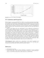
From optimization point of view, design space exploration can be distilled to
identifying a set of Pareto optimal design points according to some objective func-
tion. These design points form a curve that provides the best tradeoffs for the
variables in the objective function. Once the curve is constructed, the designer can
make design decisions based on the relative merits of the various system configu-
rations. Timing performance and the hardware cost are two common objectives in
such process.
Resource allocation and scheduling are two fundamental problems in construct-
ing such Pareto optimal curves for time/cost tradeoffs. By applying resource con-
strained scheduling, we try to minimize the application latency without violating
the resource constraints. Here allocation is performed before scheduling, and a dif-
ferent resource allocation will likely produce a vastly different scheduling result.
On the other hand, we could perform scheduling before allocation; this is the time
constrained scheduling problem. Here the inputs are a data flow graph and a time
deadline (latency). The output is again a start time for each operation, such that the
latency is not violated, while attempting to minimize the number of resources that