12 High-Level Synthesis of Loops Using the Polyhedral Model 219
In Sect. 12.3, we shall survey the front-end transformations whereas back-end
will be presented in Sect. 12.4.
12.3 The MMAlpha Front-End: From Initial Specifications
to a Virtual Architecture
The front-end of MMAlpha contains several tools to perform code analysis and
transformations.
Code analysis and verification: The initial specification of the program, called
here a loop nest, is translated into an internal representation in form of recurrence
equations. Thanks to the polyhedral model, some properties of the loop nest can
be checked by analysis: one can check for example that all elements of an array
(represented by an A
LPHA variable) are defined and used in a system, by means
of calculations on domains. More complex properties of code can also be checked
using verification techniques [8].
Scheduling: This is the central step of MMAlpha. It consists in analyzing the
dependences between the variables, and deriving for each variable, say V[i,j]
a timing-function t
V
(i, j) which gives the time instant at which this variable
can be computed. Timing-functions are usually affine, of the form t
V
(i, j)=
α
V
i+
β
V
j+
γ
V

with coefficients depending on variable V. Finding out a schedule
is performed by solving an integer linear problem using parameterized integer
programming and is described in [17]. More complex schedules can be found:
multi-dimensional timing functions, for example, allow some forms of loop tiling
to be represented, but code generation is still not available for such functions.
Localization: It is an optional transformation (also sometimes referred to as
uniformization or pipelining) that helps removing long interconnections [28].
It is inherited from the theory of systolic arrays where data which are re-
used in a calculation should be read only once from memory, thus saving
input–outputs. MMAlpha performs automatically many such localization trans-
formations described in the literature.
Space–time mapping: Once a schedule is found, the system of recurrence equa-
tions is rewritten by transforming indexes of each variable, say V[i,j],inanew
reference index set V[t,p] where t is the schedule of the variable instance and p
is the processor where it can be executed. The space–time mapping amounts for-
mally to a change of basis of the domain of each variable. Finding out the basis is
done by algebraic methods described in the literature (unimodular completion).
Simple heuristics are incorporated in MMAlpha to discover quickly reasonable,
if not always optimal, changes of basis.
After front-end processing, the initial A
LPHA specification becomes a virtual
architecture where each equation can be interpreted in term of hardware. To illus-
trate this, consider a sketch of the virtual architecture produced by the front-end
from the string alignment specification as shown in Fig. 12.4. In this program, only
220 S. Derrien et al.
system sequence :{X,Y | 3<=X<=Y-1}
(QS : {i | 1<=i<=X} of integer;
DB : {j | 1<=j<=Y} of integer)
returns (res : {j | 1<=j<=Y} of integer);
var

QQS_In : {t,p | 2p-X+1<=t<=p+1; 1<=p} of integer;

M : {t,p | p<=t<=p+Y; 0<=p<=X} of integer;

let

M[t,p] =
case
{|p=0}:0;
{ | t=p; 1<=p} : 0;
{ | p+1<=t; 1<=p} :
Max4( 0[],
M[t-1,p] - 8,
M[t-1,p-1] - 8,
M[t-2,p-1] + MatchQ[t,p] );
esac;
QQS[t,p] =
case
{ | t=p+1} : QQS_In;
{ | p+2<=t} : QQS[t-1,p];
esac;

tel;
Fig. 12.4 Sketch of the virtual parallel architecture produced by the front-end of MMAlpha. Only
variables M and QQS are represented. Variable QQS was produced by localization to propagate the
query sequence to each cell of this array
the declaration and the definition of variable M (present in the initial program) and
of a new QQS variable are kept. In the declaration of M, we can see that the domain
of this variable in now indexed by t and p. The constraints on these indexes let us
infer that the calculation of this variable is going to be done on a linear array of

X +1 processors. The definition of M reveals several informations. It shows that the
calculation of M[t,p] is the maximum of four quantities: the constant 0, the pre-
vious value M[t-1,p] which can be interpreted as a register in processor p,the
previous value M[t-1,p-1] which was held in neighboring processor p −1, and
value M[t-2,p-1],alsoheldinprocessorp −1. All these informations can be
directly interpreted in term of hardware elements. However, the linear inequalities
guarding the branches of this definition are much less straightforward to translate
into hardware. Moreover, the number of processors of this architecture is directly
linked to the size parameter X, which may not be appropriate for the requirements
of a practical application: this is the rˆole of the back-end of MMAlpha to trans-
form this virtual architecture into a real one. The QQS variable requires some more
12 High-Level Synthesis of Loops Using the Polyhedral Model 221
explanations, as it is not present in the initial specification. It is produced by the
localization transformation, in order to propagate the query value QS from proces-
sor to processor. A careful examination of its declaration and its definition reveals
that this variable is present only in processors 1 to X and initialized by reading the
value of another variable QQS
In when t = p+ 1, otherwise, it is kept in a register
of processor p.AsforM, the guards of this equation must be translated into simpler
hardware elements.
12.4 The Back-End Process: Generating VHDL
The back-end of MMAlpha comprises a set of transformations allowing a vir-
tual parallel architecture to be transformed into a synthesizable
VHDL descrip-
tion. These transformations can be regrouped into three parts (see Fig. 12.3):
hardware-mapping, structured
HDL Generation, and VHDL generation.
In this section, we review these back-end transformations as they are imple-
mented in MMAlpha by highlighting the concepts underlying them rather than the
implementation details.

12.4.1 Hardware-Mapping
The virtual architecture is essentially an operational parallel description of the
initial specification: each computation occurs at a particular date on a particular pro-
cessor. The two main transformations needed to obtain an architectural description
are: control signal generation and simple expression generation. They are imple-
mented in the hardware-mapping component which produces a subset of A
LPHA
traditionally referred to as ALPHA0.
12.4.1.1 Control Signal Generation
It consists in replacing complex, linear inequalities by the propagation of simple
control signals and is better explained here on an example. Consider for instance
the definition of the QQS variable in the program of Fig. 12.4. It can be interpreted
as a multiplexer controlled by a signal which is true at step t=p in processor number
p (Fig. 12.5a). It is easy to see intuitively that this control can be implemented by
a signal initialized in the first processor (i.e., value 1 at step 0 in processor 0) and
then transmitted to the neighboring processor with a one cycle delay (i.e., value 1
at step 1 in processor 1, and so on). This is illustrated on Fig. 12.5b: the control
signal QQS
ctl is inferred and is pipelined through the array. This is what the
control signal generation achieves: to produce a particular cell (the controller)at
the boundary of the regular array and to pipeline (or broadcast) this control signal
through the array.
222 S. Derrien et al.
Max
QQS
t == p
Proc p
Mux
QQS_In
Max

QQS_ctrl
QQS_In
QQS
Proc p
Mux
a) b)
Fig. 12.5 Control signal inference for QQS updating
QQSReg6[t,p] = QQS[t-1,p];
QQS_In[t,p] = QQSReg6[t,p-1];
QQS[t,p] =
case
{ | 1<=p<=X;} : if (QQSXctl1) then
case
{ | t=p+1;} : QQS_In;
{ | p+2<=t<=p+Y;} : 0[];
esac else
case
{ | t=p+1; } : 0[];
{ | p+2<=t<=p+Y; } : QQSReg6;
esac;
esac;
1
2
3
4
5
6
7
8
9

10
11
12
13
14
Fig. 12.6 DescriptioninALPHA0 of the hardware of Fig. 12.5b
12.4.1.2 Generation of Simple Expressions
This transformation deals with splitting complex equations in several simpler equa-
tions so that each one corresponds to a single hardware component: a register, an
operator or a simple wire.
In the A
LPHA0 subset of ALPHA,theRTL architecture can be very easily deduced
from the code. For instance Fig. 12.6 shows three equations which represent: a reg-
ister (line 1), a connexion between two processors (line 2) and a multiplexer (lines
3–14). They are interconnected to produce the hardware shown in Fig. 12.5b.
12.4.2 Structured HDL Generation
The second step of the back-end deals with generating a structured hardware
description from the A
LPHA0 format so that the re-use of identical cells explicitly
appears in the structuration of the program and provision is made to include other
components in the description. The subset of A
LPHA whichisusedatthislevelis
called A
LPHARD and is illustrated in Fig. 12.7. Here, we have a module including
12 High-Level Synthesis of Loops Using the Polyhedral Model 223
Cell B
Cell B
Module
Start
clk


Module CCell A
Inputs Outputs
clk−enable
Controller
reset
Cell B
Fig. 12.7 An ALPHARD program is a complex module containing a controller and various
instantiations of cells or modules
a local controller, a single instance of a A cell, several instances of a B cell and an
instance of another module. Cells are simple data-paths whereas modules include
controllers and can instantiate other cells and modules. Thanks to the hierarchical
structure of A
LPHA, it is easy to represent such a system in our language while
keeping its semantics.
In the case of the string alignment application, the hardware structure contains,
in addition to the controller, an instance of a particular cell representing processor
p = 0, and X −1 instances of another cell representing processors 1 to X.Itis
depicted in Fig. 12.8. (for the sake of clarity the controller and the control signal are
not represented).
The main difficulty of this step is to uncover, in the set of recurrence equations
of A
LPHA0, the least number of common cells. To this end, the polyhedral domains
of all equations are projected on the space indexes and combined to form space
maximal regions sharing the same behavior. Each such region defines a cell of the
architecture. This operation is made possible thanks to the polyhedral model which
allows projection, intersection, unions, etc. of domains to be computed easily.
12.4.3 Generating VHDL
The VHDL generation is basically a syntax-directed translation of the ALPHARD
program as each ALPHA construct corresponds to a VHDL construct. For instance,

the
VHDL code that corresponds to the ALPHA0 code shown in Fig. 12.6 is given
in Fig. 12.9. Line 1 is a simple connexion, line 3 represents a multiplexer and lines
5–8 model a register. One can notice that the time index t disappears (except in the
controller) as it is implemented by the clk and a clock enable signal.
If the variable sizes are not specified in the A
LPHA program, the translator
assumes 16-bit fixed-point arithmetics (using std
logic vector VHDL type)
but other signal types can be specified.
VHDL test benches are also generated to ease
the testing of the resulting
VHDL.
224 S. Derrien et al.
!"#
!"#
!"#
!"#
!"#
!"#
!"#
!"#
!"#
!"#
!"#
!"#
!"#
!"#
!"#
!"#

!"#
!"#
!"#
!"#
!"#
!"#
!"#
!"#
!"#
!"#
!"#
15
8
8
8
8
0
0
_
12
15
_
12
15
_
12
!)#
!)#
!)#!)#
-

-
-
!)#
-
!)#
,
!)#
,
Proc 0
Proc 1
Proc X
M
QS
DB
Mux Mux
Mux
Mux
Mux
MuxMux
Mux
+
+
X−1 times
=
8
8
+
+
+
0

Fig. 12.8 Architecture of the string matching application
12 High-Level Synthesis of Loops Using the Polyhedral Model 225
QQS_In <= QQSReg6_In;
QQS <= QQS_In WHEN QQSXctl1 =
‘1’ ELSE QQSReg6;
PROCESS(clk) BEGIN IF (clk =
‘1’ AND clk’EVENT) THEN
IF CE=
‘1’ THEN QQSReg6 <= QQS; END IF;
END IF;
END PROCESS;
1
2
3
4
5
6
7
8
Fig. 12.9 VHDL code corresponding to the ALPHA0 code shown in Fig. 12.6
12.5 Partitioning for Resource Management
In MMAlpha, the choice of the various scheduling and/or space–time mappings can
be seen as a design space exploration step. However there are practical situations in
which none of the virtual architectures obtained through the flow matches the user
requirements. This is often the case when iteration domains involved in the loop
nests are very wide: in such situations, the mapping may result in an architecture
with a very large number of processing elements, which often exceeds the allowed
silicon budget. As an example, assuming a string alignment program with a query
size X = 10
3

, the architecture corresponding to the mapping proposed in Sect. 12.3
and shown in Fig. 12.4 would result in 10
3
processing elements, which represents a
huge cost in term of hardware resources.
Many methods can be used to overcome such a difficulty. In the context of regular
parallel architectures, partitioning transformations are the method of choice. Here,
we consider a processor array partitioning transformation, which can be applied
directly on the virtual architecture (i.e., at the RTL level).
Partitioning is a well studied problem [14, 25] and it is essentially based on
the combination of two techniques. Locally Sequential Globally Parallel (LSGP)
partitioning consists in merging several virtual PE into a single PE with modi-
fied time-sliced schedule. Locally Parallel Globally Sequential (LPGS) partitioning
consists in tiling the virtual processor array into a set of virtual sub-arrays, and in
executing the whole computations as a sequence of passes on the sub-array.
In the following, we present an LSGP technique based on serialization [13]:
serialization merges
σ
virtual processors along a given processor axis into a single
physical processor. One can show that a complete LSGP partitioning can be obtained
through the use of successive serializations along the processor space axis.
To explain the principles of serialization, consider the processor datapath of the
string alignment architecture shown in Fig. 12.10. We distinguish temporal registers
(shown in grey) which have both their source and sink in the same processor, and
spatial registers, the source and sink of which are in distinct processors. (We assume
that registers have always a single sink, which is easy to ensure by transformation if
needed.) Besides we assume that the communications between processing elements
are unidirectional and pipelined.
226 S. Derrien et al.
Max

15
−12
8
8
0
i,j
i,j
M
DB
QS
M
i,j
i,j
i,j
i,j
i,j
QS
M
DB
i,j
M
mux
=
mux
max
+
max
max
sub sub
Fig. 12.10 Original datapath of the string alignment processor

Under these assumptions, serialization can be done in two steps:
– Any temporal register is transformed into a shift register line of depth
σ
.
– A one cycle delay feedback loop is associated to each spatial register; this feed-
back loop is controlled (through an additional multiplexer) by a signal activated
every
σ
cycles.
Obviously, a serialization by a factor
σ
replaces an array of X processors by
a partitioned array containing X/
σ
 processors. Figure 12.11 shows the effect of
a serialization with
σ
= 3. This kind of transformation can be used to adjust the
number of processors to the needs of the application. It can also be combined with
various other transformations to cover a large set of potential hardware configura-
tions. An example of hardware resource exploration for a bioinformatics application
is presented in [11].
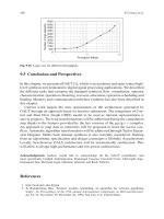
12.6 Implementation and Performance
To illustrate the typical performance of a parallel implementation of an applica-
tion, we implemented on a Xilinx Virtex-4 device several configurations of string
alignment with or without partitioning. The results are shown in Table 12.1. For
each configuration, the number X of processors, the total resources of the device,
– look-up tables, flip-flops and number of slices – the clock frequency and the
performance, in Giga Cell Update per second (GCUps) are given. The last four
lines present partitioned versions. As a reference, we show the typical performance

of a software implementation of the string aligment on a desktop computer which
12 High-Level Synthesis of Loops Using the Polyhedral Model 227
Max
8
8
0
−12
15
M
=
mux
i,j
i,j
QS
M
DB
i,j
mux
DB
QS
i,j
i,j
mux
mux
sub sub
i,j
i,j
M
M
mux

max
+
max
max
i,j
Fig. 12.11 The string alignment processor datapath after serialization by
σ
= 3
Table 12.1 Performance of various string alignment hardware configurations measured in Giga
Cell Updates per seconds
Description LUT/DFF/Slices Clock (MHz) Perf. (GCUps)
Software – – 0, 1
X = 10 1,047/1,619/1,047 110 1.1
X = 50 8,088/4,130/4,771 110 5.5
X = 100 16,300/8,233/9,542 110 11
X = 100,
σ
= 210.8K/4,308/6,628 95 5.5
X = 100,
σ
= 10 2K/1K/1,543 102 ≈1.0
X = 100,
σ
= 20 1.2K/550/931 93 ≈0.45
X = 100,
σ
= 50 5.6K/231/517 98 ≈0.2
LU T is the number of look-up tables, DFF is the number of data flip-flops,
and Slices is the number of Virtex-4
FPGA slices used by the designs

achieves 100MCUps. The speed-up factor reaches up to two orders of magnitude
depending on the number of processors. It is also noteworthy that the derived archi-
tecture is scalable: the achievable clock period does not suffer from an increase in
the number of processing elements, and the hardware resource cost grows linearly
with that number.
12.7 Other Works: The Polyhedral Model
The polyhedral model has been used for memory modeling [9, 15], communi-
cation modeling [33], cache misses [24], but its most important use was done in
parallelizing compilers and
HLS tools.
228 S. Derrien et al.
There is an important trend in commercial high-level synthesis tools to perform
hardware synthesis from C programs: CatapultC (Mentor Graphics), Pico (Syn-
fora) [30], Cynthesizer (Forte Design System) [18], and Cascade (Critical Blue) [4].
However all these tools suffer from inefficient handling of arbitrary nested loops
algorithms.
Academic
HLS tools are numerous and reflect the focus of recent researches on
efficient synthesis of application-specific algorithms. Among the most important
tools: Spark [19], Compaan/Laura [32], ESPAM [27], MMAlpha [26], Paro [6],
Gaut [31],
UGH [2], Streamroller [22], xPilot [7]. Compaan, Paro and MMAlpha
have focused of the efficient compilation of loops, and they use the polyhedral
model to perform loop analysis and/or transformations. Another formalism, called
Array-OL, has been used for multidimensional signal processing [10] and revisited
recently [5].
Parallelizing compiler prototypes have also provided a lot of research results on
loop transformations [23]: Tiny [34], LooPo [20], Suif [1] or Pips [21]. Recently,
WraPit [3], integrated in the Open64 compiler, proposed an explicit polyhedral
internal representation for loop nest, very close to the representation used by

MMAlpha.
12.8 Conclusion
We have shown the main principles of high-level synthesis for loops targeting par-
allel architectures. Our presentation has used the MMAlpha tools as an example to
explain the polyhedral model, the basic loops transformations, and the way these
transformations may be arranged in order to produce parallel hardware. MMAlpha
uses the A
LPHA single-assignment language to represent the architecture, from its
initial specification to its practical, synthesizable hardware implementation.
The polyhedral model, which underlies the representation and transformation of
loops, is a very powerful vehicle to express the variety of transformations that can
be used to extract parallelism et take benefit of it for hardware implementations.
Future SoC architectures will increasingly need such techniques to exploit available
multi-core architectures. We therefore believe that it is a good basis for carrying
research on HLS whenever parallelism is considered.
References
1. S. Amarasinghe et al. Suif: An Infrastructure for Research on Parallelizing and Optimizing
Compilers. Technical report, Stanford University, May 1994.
2. I. Aug´e, F. P´etrot, F. Donnet, and P. Gomez. Platform-Based Design From Parallel C Speci-
fications. IEEE Transactions on Computer-Aided Design of Integrated Circuits and Systems,
24(12):1811–1826, 2005.
3. C. Bastoul, A. Cohen, S. Girbal, S. Sharma, and O. Temam. Putting Polyhedral Loop
Transformations to Work. In LCPC, pages 209–225, 2003.