2752 ✦ Chapter 43: Using Predictor Variables
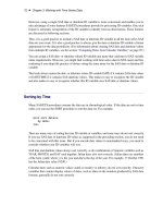
Figure 43.11 Dynamic Regressors Selection Window
You can select only one predictor series when specifying a dynamic regression model. For this
example, select VEHICLES, Sales: Motor Vehicles and Parts. Then select the OK button.
This displays the Dynamic Regression Specification window, as shown in Figure 43.12.
Dynamic Regressor ✦ 2753
Figure 43.12 Dynamic Regression Specification Window
This window consists of four parts. The
Input Transformations
fields enable you to transform
or lag the predictor variable. For example, you might use the lagged logarithm of the variable as the
predictor series.
The
Order of Differencing
fields enable you to specify simple and seasonal differencing of the
predictor series. For example, you might use changes in the predictor variable instead of the variable
itself as the predictor series.
The
Numerator Factors
and
Denominator Factors
fields enable you to specify the orders of
simple and seasonal numerator and denominator factors of the transfer function.
Simple regression is a special case of dynamic regression in which the dynamic regression model
consists of only a single regression coefficient for the current value of the predictor series. If you
select the
OK
button without specifying any options in the Dynamic Regression Specification window,
a simple regressor will be added to the model.
For this example, use the
Simple Order

combo box for
Denominator Factors
and set its value
to 1. The window now appears as shown in Figure 43.13.
2754 ✦ Chapter 43: Using Predictor Variables
Figure 43.13 Distributed Lag Regression Specified
This model is equivalent to regression on an exponentially weighted infinite distributed lag of
VEHICLES (in the same way an MA(1) model is equivalent to single exponential smoothing).
Select the OK button to add the dynamic regressor to the model predictors list.
In the ARIMA Model Specification window, the Predictors list should now contain two items, a
linear trend and a dynamic regressor for VEHICLES, as shown in Figure 43.14.
Interventions ✦ 2755
Figure 43.14 Dynamic Regression Model
This model is a multiple regression of PETROL on a time trend variable and an infinite distributed
lag of VEHICLES. Select the OK button to fit the model.
As with simple regressors, if VEHICLES does not already have a forecasting model, an automatic
model selection process is performed to find a forecasting model for VEHICLES before the dynamic
regression model for PETROL is fit.
Interventions
An intervention is a special indicator variable, computed automatically by the system, that identifies
time periods affected by unusual events that influence or intervene in the normal path of the time
series you are forecasting. When you add an intervention predictor, the indicator variable of the
intervention is used as a regressor, and the impact of the intervention event is estimated by regression
analysis.
To add an intervention to the Predictors list, you must use the Intervention Specification window to
specify the time or times that the intervening event took place and to specify the type of intervention.
2756 ✦ Chapter 43: Using Predictor Variables
You can add interventions either through the
Interventions
item of the

Add
action or by selecting
Tools from the menu bar and then selecting Define Interventions.
Intervention specifications are associated with the series. You can specify any number of interventions
for each series, and once you define interventions you can select them for inclusion in forecasting
models. If you select the
Include Interventions
option in the
Options
menu, any interventions
that you have previously specified for a series are automatically added as predictors to forecasting
models for the series.
From the Develop Models window, invoke the series viewer by selecting the
View Series
Graphically
icon or
Series
under the
View
menu. This displays the Time Series Viewer, as
was shown in Figure 43.2.
Note that the trend in the PETROL series shows several clear changes in direction. The upward trend
in the first part of the series reverses in 1981. There is a sharp drop in the series towards the end of
1985, after which the trend is again upwardly sloped. Finally, in 1991 the series takes a sharp upward
excursion but quickly returns to the trend line.
You might have no idea what events caused these changes in the trend of the series, but you can use
these patterns to illustrate the use of intervention predictors. To do this, you fit a linear trend model
to the series, but modify that trend line by adding intervention effects to model the changes in trend
you observe in the series plot.
The Intervention Specification Window

From the Develop Models window, select
Fit ARIMA
model. From the ARIMA Model Specification
window, select Add and then select Linear Trend from the menu (shown in Figure 43.1).
Select
Add
again and then select
Interventions.
If you have any interventions already defined for
the series, this selection displays the
Interventions for Series
window. However, since you
have not previously defined any interventions, this list is empty. Therefore, the system assumes that
you want to add an intervention and displays the
Intervention Specification
window instead,
as shown in Figure 43.15.
The Intervention Specification Window ✦ 2757
Figure 43.15 Interventions Specification Window
The top of the Intervention Specification window shows the current series and the label for the new
intervention (initially blank). At the right side of the window is a scrollable table showing the values
of the series. This table helps you locate the dates of the events you want to model.
At the left of the window is an area titled
Intervention Specification
that contains the options
for defining the intervention predictor. The
Date
field specifies the time that the intervention occurs.
You can type a date value in the
Date

field, or you can set the Date value by selecting a row from the
table of series values at the right side of the window.
The area titled
Type of Intervention
controls the kind of indicator variable constructed to model
the intervention effect. You can specify the following kinds of interventions:
Point
is used to indicate an event that occurs in a single time period. An example of a
point event is a strike that shuts down production for part of a time period. The
value of the intervention’s indicator variable is zero except for the date specified.
Step
is used to indicate a continuing event that changes the level of the series. An
example of a step event is a change in the law, such as a tax rate increase. The
value of the intervention’s indicator variable is zero before the date specified and
1 thereafter.
2758 ✦ Chapter 43: Using Predictor Variables
Ramp
is used to indicate a continuing event that changes the trend of the series. The
value of the intervention’s indicator variable is zero before the date specified, and
it increases linearly with time thereafter.
The areas titled
Effect Time Window
and
Effect Decay Pattern
specify how to model the
effect that the intervention has on the dependent series. These options are not used for simple
interventions, they will be discussed later in this chapter.
Specifying a Trend Change Intervention
In the Time Series Viewer window position the mouse over the highest point in 1981 and select the
point. This displays the data value, 19425, and date, February 1981, of that point in the upper-right

corner of the Time Series Viewer, as shown in Figure 43.16.
Figure 43.16 Identifying the Turning Point
Now that you know the date that the trend reversal occurred, enter that date in the
Date
field of the
Intervention Specification window. Select
Ramp
as the type of intervention. The window should now
appear as shown in Figure 43.17.
Specifying a Trend Change Intervention ✦ 2759
Figure 43.17 Ramp Intervention Specified
Select the
OK
button. This adds the intervention to the list of interventions for the PETROL series,
and returns you to the Interventions for Series window, as shown in Figure 43.18.
2760 ✦ Chapter 43: Using Predictor Variables
Figure 43.18 Interventions for Series Window
This window allows you to select interventions for inclusion in the forecasting model. Since you need
to define other interventions, select the
Add
button. This returns you to the Intervention Specification
window (shown in Figure 43.15).
Specifying a Level Change Intervention
Now add an intervention to account for the drop in the series in late 1985. You can locate the date of
this event by selecting points in the Time Series Viewer plot or by scrolling through the data values
table in the Interventions Specification window. Use the latter method so that you can see how this
works.
Scrolling through the table, you see that the drop was from 15262 in December 1985, to 13937 in
January 1986, to 12002 in February, to 10834 in March. Since the drop took place over several
periods, you could use another ramp type intervention. However, this example represents the drop as

a sudden event by using a step intervention and uses February 1986 as the approximate time of the
drop.
Modeling Complex Intervention Effects ✦ 2761
Select the table row for February 1986 to set the
Date
field. Select
Step
as the intervention type.
The window should now appear as shown in Figure 43.19.
Figure 43.19 Step Intervention Specified
Select the OK button to add this intervention to the list for the series.
Since the trend reverses again after the drop, add a ramp intervention for the same date as the step
intervention. Select
Add
from the Interventions for Series window. Enter FEB86 in the
Date
field,
select Ramp, and then select the OK button.
Modeling Complex Intervention Effects
You have now defined three interventions to model the changes in trend and level. The excursion
near the end of the series remains to be dealt with.
Select
Add
from the Interventions for Series window. Scroll through the data values and select the
date on which the excursion began, August 1990. Leave the intervention type as Point.