2722 ✦ Chapter 42: Choosing the Best Forecasting Model
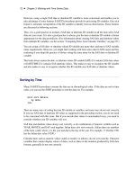
Figure 42.3 Selecting an Area for Zoom
The zoomed plot should appear as shown in Figure 42.4.
Time Series Viewer Features ✦ 2723
Figure 42.4 Zoomed Plot
You can repeat the process to zoom in still further. To return to the previous view, select the Zoom
Out icon, the second icon on the window’s horizontal toolbar.
The third icon on the horizontal toolbar is used to link or unlink the viewer window. By default,
the viewer is linked, meaning that it is automatically updated to reflect selection of a different time
series. To see this, return to the Series Selection window by clicking on it or using the Window
menu or
Next Viewer
toolbar icon. Select the Electric series in the
Time Series Variables
list box. Notice that the Time Series Viewer window is updated to show a plot of the ELECTRIC
series. Select the
Link/Unlink
icon if you prefer to unlink the viewer so that it is not automatically
updated in this way. Successive selections toggle between the linked and unlinked state. A note on
the message line informs you of the state of the Time Series Viewer window.
When a Time Series Viewer window is linked, selecting
View Series
again makes the linked
Viewer window active. When no Time Series Viewer window is linked, selecting
View Series
opens an additional Time Series Viewer window. You can bring up as many Time Series Viewer
windows as you want.
Having seen the plot in Figure 42.2, you might suspect that the series is nonstationary and seasonal.
You can gain further insight into this by examining the sample autocorrelation function (ACF), partial
autocorrelation function (PACF), and inverse autocorrelation function (IACF) plots. To switch the
2724 ✦ Chapter 42: Choosing the Best Forecasting Model

display to the autocorrelation plots, select the second icon from the top on the vertical toolbar at the
right side of the Time Series Viewer. The plot appears as shown in Figure 42.5.
Figure 42.5 Sample Autocorrelation Plots
Each bar represents the value of the correlation coefficient at the given lag. The overlaid lines
represent confidence limits computed at plus and minus two standard errors. You can switch the
graphs to show significance probabilities by selecting
Correlation Probabilities
under the
Options pull-down menu, or by selecting the Toggle ACF Probabilities toolbar icon.
The slow decline of the ACF suggests that first differencing might be warranted. To see the effect
of first differencing, select the simple difference icon, the fifth icon from the left on the window’s
horizontal toolbar. The plot now appears as shown in Figure 42.6.
Time Series Viewer Features ✦ 2725
Figure 42.6 ACF Plots with First Difference Applied
Since the ACF still displays slow decline at seasonal lags, seasonal differencing is appropriate (in
addition to the first differencing already applied). Select the
Seasonal Difference
icon, the sixth
icon from the left on the horizontal toolbar. The plot now appears as shown in Figure 42.7.
2726 ✦ Chapter 42: Choosing the Best Forecasting Model
Figure 42.7 ACF Plot with Simple and Seasonal Differencing
Model Viewer Prediction Error Analysis
Leave the Time Series Viewer open for the remainder of this exercise. Drag it out of the way or
push it to the background so that you can return to the Time Series Forecasting window. Select
Develop Models
, then click an empty part of the table to bring up the pop-up menu, and select
Fit ARIMA Model
. Define the
ARIMA(0,1,0)(0,1,0)s
model by selecting

1
for Differencing under
ARIMA Options,
1
for Differencing under Seasonal ARIMA Options, and
No
for
Intercept
, as
shown in Figure 42.8.
Model Viewer Prediction Error Analysis ✦ 2727
Figure 42.8 Specifying the ARIMA(0,1,0)(0,1,0)s Model
When you select the
OK
button, the model is fit and you are returned to the Develop Models
window. Click on an empty part of the table and choose
Fit Models from List
from the pop-
up menu. Select
Airline Model
from the window. (Airline Model is a common name for the
ARIMA(0,1,1)(0,1,1)s model, which is often used for seasonal data with a linear trend.) Select the
OK
button. Once the model has been fit, the table shows the two models and their root mean square
errors. Notice that the Airline Model provides only a slight improvement over the differencing
model, ARIMA(0,1,0)(0,1,0)s. Select the first row to highlight the differencing model, as shown in
Figure 42.9.
2728 ✦ Chapter 42: Choosing the Best Forecasting Model
Figure 42.9 Selecting a Model
Now select the

View Selected Model Graphically
button, below the
Browse
button at the right
side of the Develop Models window. The
Model Viewer
window appears, showing the actual data
and model predictions for the MASONRY series. (Note that predicted values are missing for the first
13 observations due to simple and seasonal differencing.)
To examine the ACF plot for the model prediction errors, select the third icon from the top on the
vertical toolbar. For this model, the prediction error ACF is the same as the ACF of the original data
with first differencing and seasonal differencing applied. This differencing is apparent if you bring
the Time Series Viewer back into view for comparison.
Return to the Develop Models Window by clicking on it or using the window pull-down menu or
the Next Viewer toolbar icon. Select the second row of the table in the Develop Models window to
highlight the Airline Model. The Model Viewer is automatically updated to show the prediction error
ACF of the newly selected model, as shown in Figure 42.10.
Model Viewer Prediction Error Analysis ✦ 2729
Figure 42.10 Prediction Error ACF Plot for the Airline Model
Another helpful tool available within the Model Viewer is the parameter estimates table. Select the
fifth icon from the top of the vertical toolbar. The table gives the parameter estimates for the two
moving-average terms in the Airline Model, as well as the model residual variance, as shown in
Figure 42.11.
2730 ✦ Chapter 42: Choosing the Best Forecasting Model
Figure 42.11 Parameter Estimates for the Airline Model
You can adjust the column widths in the table by dragging the vertical borders of the column titles
with the mouse. Notice that neither of the parameter estimates is significantly different from zero at
the 0.05 level of significance, since
Prob>|t|
is greater than 0.05. This suggests that the Airline

Model should be discarded in favor of the more parsimonious differencing model, which has no
parameters to estimate.
The Model Selection Criterion
Return to the Develop Models window (Figure 42.9) and notice the Root Mean Square Error button
at the right side of the table banner. This is the model selection criterion—the statistic used by the
system to select the best fitting model. So far in this example you have fit two models and have left
the default criterion, root mean square error (RMSE), in effect. Because the Airline Model has the
smaller value of this criterion and because smaller values of the RMSE indicate better fit, the system
has chosen this model as the forecasting model, indicated by the check box in the
Forecast Model
column.
The Model Selection Criterion ✦ 2731
The statistics available as model selection criteria are a subset of the statistics available for infor-
mational purposes. To access the entire set, select
Options
from the menu bar, and then select
Statistics of Fit.
The
Statistics of Fit Selection
window appears, as shown in Fig-
ure 42.12.
Figure 42.12 Statistics of Fit
By default, five of the more well known statistics are selected. You can select and deselect statistics by
clicking the check boxes in the left column. For this exercise, select
All
, and notice that all the check
boxes become checked. Select the
OK
button to close the window. Now if you choose
Statistics

of Fit in the Model Viewer window, all of the statistics will be shown for the selected model.
To change the model selection criterion, click the
Root Mean Square Error
button or select
Options
from the menu bar and then select
Model Selection Criterion.
Notice that most
of the statistics of fit are shown, but those which are not relevant to model selection, such as
number of observations, are not shown. Select
Schwarz Bayesian Information Criterion
and click
OK
. Since this statistic puts a high penalty on models with larger numbers of parameters,
the ARIMA(0,1,0)(0,1,0)s model comes out with the better fit.
Notice that changing the selection criterion does not automatically select the model that is best
according to that criterion. You can always choose the model you want to use for forecasts by
selecting its check box in the Forecast Model column.