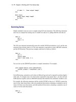
SAS/ETS 9.22 User''''s Guide 271 pptx
Bạn đang xem bản rút gọn của tài liệu. Xem và tải ngay bản đầy đủ của tài liệu tại đây (623.31 KB, 10 trang )
2692 ✦ Chapter 41: Specifying Forecasting Models
Figure 41.11 Transformation Options
You can specify a logarithmic, logistic, square root, or Box-Cox transformation. For this example,
select “Square Root” from the list. The Transformation field is now set to Square Root.
This means that the system will first take the square roots of the series values, apply the additive
version of the Winters method to the square root series, and then produce the predictions for the
original series by squaring the Winters method predictions (and multiplying by a variance factor if
the Mean Prediction option is set in the Forecast Options window). See Chapter 46, “Forecasting
Process Details,” for more information about predictions from transformed models.
The Smoothing Model Specification window should now appear as shown in Figure 41.12. Select the
OK button to fit the model. The model is added to the table of fitted models in the Develop Models
window.
ARIMA Model Specification Window ✦ 2693
Figure 41.12 Winter’s Method Applied to Square Root Series
ARIMA Model Specification Window
To fit ARIMA or Box-Jenkins models not already provided in the Models to Fit window, select the
ARIMA model item from the pop-up menu, toolbar, or Edit menu. This opens the ARIMA Model
Specification window, as shown in Figure 41.13.
2694 ✦ Chapter 41: Specifying Forecasting Models
Figure 41.13 ARIMA Model Specification Window
This ARIMA Model Specification window is structured according to the Box and Jenkins approach
to time series modeling. You can specify the same time series models with the Custom Model
Specification window and the ARIMA Model Specification window, but the windows are structured
differently, and you may find one more convenient than the other.
At the top of the ARIMA Model Specification window is the name and label of the series and the
label of the model you are specifying. The model label is filled in with an automatically generated
label as you specify options. You can type over the automatic label with your own label for the
model. To restore the automatic label, enter a blank label.
Using the ARIMA Model Specification window, you can specify autoregressive (p), differencing (d),
and moving average (q) orders for both simple and seasonal factors. You can specify transformations
with the
Transformation
list. You can also specify whether an intercept is included in the ARIMA
model.
In addition to specifying seasonal and nonseasonal ARIMA processes, you can also specify predictor
variables and other terms as inputs to the model. ARIMA models with inputs are sometimes called
ARIMAX models or Box-Tiao models. Another term for this kind of model is dynamic regression.
In the lower part of the ARIMA Model Specification window is the list of predictors to the model
(initially empty). You can specify predictors by using the Add button. This opens a menu of different
kinds of independent effects, as shown in Figure 41.14.
ARIMA Model Specification Window ✦ 2695
Figure 41.14 Add Predictors Menu
The kinds of predictor effects allowed include time trends, regressors, adjustments, dynamic regres-
sion (transfer functions), intervention effects, and seasonal dummy variables. How to use different
kinds of predictors is explained in Chapter 43, “Using Predictor Variables.”
As an example, in the
ARIMA Options
box, set the order of differencing
d
to
1
and the moving
average order
q
to
2
. You can either type in these values or click the arrows and select the values
from pop-up lists.
These selections specify an ARIMA(0,1,2) or IMA(1,2) model. (See Chapter 7, “The ARIMA
Procedure,” for more information about the notation used for ARIMA models.) Notice that the
model label at the top is now
IMA(1,2) NOINT
, meaning that the data are differenced once and a
second-order moving-average term is included with no intercept.
In the
Seasonal ARIMA Options
box, set the seasonal moving-average order
Q
to
1
. This adds
a first-order moving-average term at the seasonal (12 month) lag. Finally, select “Log” in the
Transformation combo box.
The model label is now
Log ARIMA(0,1,2)(0,0,1)s NOINT
, and the window appears as shown
in Figure 41.15.
2696 ✦ Chapter 41: Specifying Forecasting Models
Figure 41.15 Log ARIMA(0,1,2)(0,0,1)s Specified
Select the OK button to fit the model. The model is fit and added to the Develop Models table.
Factored ARIMA Model Specification Window
To fit a factored ARIMA model, select the Factored ARIMA model item from the pop-up menu,
toolbar, or Edit menu. This brings up the Factored ARIMA Model Specification window, shown in
Figure 41.16.
Factored ARIMA Model Specification Window ✦ 2697
Figure 41.16 Factored ARIMA Model Specification Window
The Factored ARIMA Model Specification window is similar to the ARIMA Model Specification
window and has the same features, but it uses a more general specification of the autoregressive (p),
differencing (d), and moving-average (q) terms. To specify these terms, select the corresponding Set
button, as shown in Figure 41.16. For example, to specify autoregressive terms, select the first Set
button. This opens the AR Polynomial Specification Window, shown in Figure 41.17.
2698 ✦ Chapter 41: Specifying Forecasting Models
Figure 41.17 AR Polynomial Specification Window
To add AR polynomial terms, select the New button. This opens the Polynomial Specification
Window, shown in Figure 41.18. Specify the first lag you want to include by using the
Lag
spin box,
then select the Add button. Repeat this process, adding each lag you want to include in the current
list. All lags must be specified. For example, if you add only lag 3, the model contains only lag 3,
not 1 through 3.
As an example, add lags 1 and 3, then select the OK button. The AR Polynomial Specification
Window now shows (1,3) in the list of polynomials. Now select “New” again. Add lags 6 and 12 and
select “OK”. Now the AR Polynomial Specification Window shows (1,3) and (6,12) as shown in
Figure 41.17. Select “OK” to close this window. The Factored ARIMA Model Specification Window
now shows the factored model
p=(1,3)(6,12)
. Use the same technique to specify the q terms, or
moving-average part of the model. There is no limit to the number of lags or the number of factors
you can include in the model.
Factored ARIMA Model Specification Window ✦ 2699
Figure 41.18 Polynomial Specification Window
To specify differencing lags, select the middle Set button to open the Differencing Specification
window. Specify lags using the spin box and add them to the list with the Add button. When you
select “OK” to close the window, the differencing lags appear after
d=
in the Factored ARIMA
Specification Window, within a single pair of parentheses.
You can use the Factored ARIMA Model Specification Window to specify any model that you can
specify with the ARIMA Model and Custom Model windows, but the notation is more similar to that
of the ARIMA procedure (see Chapter 7, “The ARIMA Procedure”). Consider as an example the
classic Airline model fit to the International Airline Travel series,
SASHELP.AIR
. This is a factored
model with one moving-average term at lag one and one moving-average term at the seasonal lag,
with first-order differencing at the simple and seasonal lags. Using the ARIMA Model Specification
Window, you specify the value 1 for the q and d terms and also for the Q and D terms, which represent
the seasonal lags. For monthly data, the seasonal lags represent lag 12, since a yearly seasonal cycle
is assumed.
By contrast, the Factored ARIMA Model Specification Window makes no assumptions about
seasonal cycles. The Airline model is written as
IMA d=(1,12) q=(1)(12) NOINT
. To specify the
differencing terms, add the values 1 and 12 in the Differencing Specification Window and select OK.
Then select “New” in the MA Polynomial Specification Window, add the value 1, and select OK. To
add the factored term, select “New” again, add the value 12, and select OK. Remember to select “No”
2700 ✦ Chapter 41: Specifying Forecasting Models
in the Intercept radio box, since it is not selected by default. Select OK to close the Factored ARIMA
Model Specification Window and fit the model.
You can show that the results are the same as they are when you specify the model by using the
ARIMA Model Specification Window and when you select Airline Model from the default model
list. If you are familiar with the ARIMA Procedure (Chapter 7, “The ARIMA Procedure”), you
might want to turn on the
Show Source Statements
option before fitting the model, then examine
the procedure source statements in the log window after fitting the model.
The strength of the Factored ARIMA Specification approach lies in its ability to contruct unusual
ARIMA models, such as:
Subset models
These are models of order n, where fewer than n lags are specified. For example,
an AR order 3 model might include lags 1 and 3 but not lag 2.
Unusual seasonal cycles
For example, a monthly series might cycle two or four times per year instead of
just once.
Multiple cycles
For example, a daily sales series might peak on a certain day each week and
also once a year at the Christmas season. Given sufficient data, you can fit a
three-factor model, such as IMA d=(1) q=(1)(7)(365).
Models with high order lags take longer to fit and often fail to converge. To save time, select the
Conditional Least Squares or Unconditional Least Squares estimation method (see Figure 41.16).
Once you have narrowed down the list of candidate models, change to the Maximum Likelihood
estimation method.
Custom Model Specification Window
To fit a custom time series model not already provided in the Models to Fit window, select the
Custom Model item from the pop-up menu, toolbar, or Edit menu. This opens the Custom Model
Specification window, as shown in Figure 41.19.
Custom Model Specification Window ✦ 2701
Figure 41.19 Custom Model Specification Window
You can specify the same time series models with the Custom Model Specification window and the
ARIMA Model Specification window, but the windows are structured differently, and you might find
one more convenient than the other.
At the top of the Custom Model Specification window is the name and label of the series and the
label of the model you are specifying. The model label is filled in with an automatically generated
label as you specify options. You can type over the automatic label with your own label for the
model. To restore the automatic label, enter a blank label.
The middle part of the Custom Model Specification window consists of four fields:
Transformation
,
Trend Model
,
Seasonal Model
, and
Error Model
. These fields allow you to specify the model
in four parts. Each part specifies how a different aspect of the pattern of the time series is modeled
and predicted.
The
Predictors
list at the bottom of the Custom Model Specification window allows you to include
different kinds of predictor variables in the forecasting model. The Predictors feature for the Custom
Model Specification window is like the Predictors feature for the ARIMA Model Specification
window, except that time trend predictors are provided through the Trend Model field and seasonal
dummy variable predictors are provided through the Seasonal Model field.