SAS/ETS 9.22 User''''s Guide 268 pptx
Bạn đang xem bản rút gọn của tài liệu. Xem và tải ngay bản đầy đủ của tài liệu tại đây (612.12 KB, 10 trang )
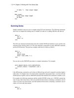
2662 ✦ Chapter 39: Getting Started with Time Series Forecasting
Figure 39.44 Model Viewer: Parameter Estimates Table
For the linear trend model, the parameters are the intercept and slope coefficients. The table shows the
values of the fitted coefficients together with standard errors and t tests for the statistical significance
of the estimates. The model residual variance is also shown.
Statistics of Fit Table
Select the sixth icon from the top in the vertical toolbar to the right of the table. This switches the
Viewer to display a table of statistics of fit computed from the model prediction errors, as shown in
Figure 39.45. The list of statistics displayed is controlled by selecting
Statistics of Fit
from
the Options menu.
Changing to a Different Model ✦ 2663
Figure 39.45 Model Viewer: Statistics of Fit Table
Changing to a Different Model
Select the first icon in the vertical toolbar to the right of the table to return the display to the predicted
and actual values plots (Figure 39.39).
Now return to the Develop Models window, but do not close the Model Viewer window. You can use
the Next Viewer icon in the toolbar or your system’s window manager controls to switch windows.
You can resize the windows to make them both visible.
Select the Double Exponential Smoothing model so that this line of the model list is highlighted.
The Model Viewer window is now updated to display a plot of the predicted values for the Double
Exponential Smoothing model, as shown in Figure 39.46. The Model Viewer is automatically
updated to display the currently selected model, unless you specify
Unlink
(the third icon in the
window’s horizontal toolbar).
2664 ✦ Chapter 39: Getting Started with Time Series Forecasting
Figure 39.46 Model Viewer Plot for Exponential Smoothing Model
Forecasts and Confidence Limits Plots
Select the seventh icon from the top in the vertical toolbar to the right of the graph. This switches the
Viewer to display a plot of forecast values and confidence limits, together with actual values and
one-step-ahead within-sample predictions, as shown in Figure 39.47.
Data Table ✦ 2665
Figure 39.47 Model Viewer: Forecasts and Confidence Limits
Data Table
Select the last icon at the bottom of the vertical toolbar to the right of the graph. This switches the
Viewer to display the forecast data set as a table, as shown in Figure 39.48.
2666 ✦ Chapter 39: Getting Started with Time Series Forecasting
Figure 39.48 Model Viewer: Forecast Data Table
To view the full data set, use the vertical and horizontal scroll bars on the data table or enlarge the
window.
Closing the Model Viewer
Other features of the Model Viewer and Develop Models window are discussed later in this book.
For now, close the Model Viewer window and return to the Time Series Forecasting window.
To close the Model Viewer window, select
Close
from the window’s horizontal toolbar or from the
File menu.
Chapter 40
Creating Time ID Variables
Contents
Creating a Time ID Value from a Starting Date and Frequency . . . . . . . . . . . . 2667
Using Observation Numbers as the Time ID . . . . . . . . . . . . . . . . . . . . . . 2671
Creating a Time ID from Other Dating Variables . . . . . . . . . . . . . . . . . . 2674
The Forecasting System requires that the input data set contain a time ID variable. If the data you
want to forecast are not in this form, you can use features of the Forecasting System to help you add
time ID variables to your data set. This chapter shows examples of how to use these features.
Creating a Time ID Value from a Starting Date and
Frequency
As a first example of adding a time ID variable, use the SAS data set created by the following
statements. (Or use your own data set if you prefer.)
data no_id;
input y @@;
datalines;
10 15 20 25 30 35 40 45
50 55 60 65 70 75 80 85
run;
Submit these SAS statements to create the data set NO_ID. This data set contains the single variable
Y. Assume that Y is a quarterly series and starts in the first quarter of 1991.
In the
Time Series Forecasting
window, use the Browse button to the right of the
Data set
field to bring up the
Data Set Selection
window. Select the WORK library, and then select the
NO_ID data set.
You must create a time ID variable for the data set. Click the Create button to the right of the Time
ID field. This opens a menu of choices for creating the Time ID variable, as shown in Figure 40.1.
2668 ✦ Chapter 40: Creating Time ID Variables
Figure 40.1 Time ID Creation Popup Menu
Select the first choice,
Create from starting date and frequency
. This opens the
Time ID
Creation from Starting Date window shown in Figure 40.2.
Creating a Time ID Value from a Starting Date and Frequency ✦ 2669
Figure 40.2 Time ID Creation from Starting Date Window
Enter the starting date, 1991:1, in the Starting Date field.
Select the
Interval
list arrow and select QTR. The Interval value QTR means that the time interval
between successive observations is a quarter of a year; that is, the data frequency is quarterly.
Now select the
OK
button. The system prompts you for the name of the new data set. If you want to
create a new copy of the input data set with the DATE variable added, enter a name for the new data
set. If you want to replace the NO_ID data set with the new copy containing DATE, just select the
OK button without changing the name.
For this example, change the
New name
field to WITH_ID and select the
OK
button. The data set
WITH_ID is created containing the series Y from NO_ID and the added ID variable DATE. The
system returns to the Data Set Selection window, which now appears as shown in Figure 40.3.
2670 ✦ Chapter 40: Creating Time ID Variables
Figure 40.3 Data Set Selection Window after Creating Time ID
Select the Table button to see the new data set WITH_ID. This opens a VIEWTABLE window for
the data set WITH_ID, as shown in Figure 40.4. Select
File
and
Close
to close the VIEWTABLE
window.
Using Observation Numbers as the Time ID ✦ 2671
Figure 40.4 Viewtable Display of Data Set with Time ID Added
Using Observation Numbers as the Time ID
Normally, the time ID variable contains date values. If you do not want to have dates associated with
your forecasts, you can also use observation numbers as time ID variables. However, you still must
have an ID variable. This can be illustrated by adding an observation index time ID variable to the
data set NO_ID.
In the Data Set Selection window, select the data set NO_ID again. Select the Create button to the
right of the
Time ID
field. Select the fourth choice,
Create from observation numbers
. This
opens the Time ID Variable Creation window shown in Figure 40.5.