1502 ✦ Chapter 22: The SEVERITY Procedure (Experimental)
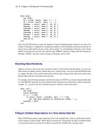
Figure 22.9 P-P Plots for the Lognormal and Weibull Models Fitted to Truncated and Censored
Data
An Example with Left-Truncation and Right-Censoring ✦ 1503
Figure 22.9 continued
Specifying Initial Values for Parameters
All the predefined distributions have parameter initialization functions built into them. For the current
example, Figure 22.10 shows the initial values that are obtained by the predefined method for the
Burr distribution. It also shows the summary of the optimization process and the final parameter
estimates.
Figure 22.10 Burr Model Summary for the Truncated and Censored Data
Initial Parameter Values and
Bounds for Burr Distribution
Initial Lower Upper
Parameter Value Bound Bound
Theta 4.78102 1.05367E-8 Infty
Alpha 2.00000 1.05367E-8 Infty
Gamma 2.00000 1.05367E-8 Infty
1504 ✦ Chapter 22: The SEVERITY Procedure (Experimental)
Figure 22.10 continued
Optimization Summary for Burr Distribution
Optimization Technique Trust Region
Number of Iterations 8
Number of Function Evaluations 21
Log Likelihood -148.20614
Parameter Estimates for Burr Distribution
Standard Approx
Parameter Estimate Error t Value Pr > |t|
Theta 4.76980 0.62492 7.63 <.0001
Alpha 1.16363 0.58859 1.98 0.0509
Gamma 5.94081 1.05004 5.66 <.0001

You can specify a different set of initial values if estimates are available from fitting the distribution
to similar data. For this example, the parameters of the Burr distribution can be initialized with the
final parameter estimates of the Burr distribution that were obtained in the first example (shown in
Figure 22.5). One of the ways in which you can specify the initial values is as follows:
/
*
Specifying initial values using INIT= option
*
/
proc severity data=test_sev2 print=(all) plots=none;
model y(lt=threshold rc=iscens(1)) / crit=aicc;
dist burr init=(theta=4.62348 alpha=1.15706 gamma=6.41227);
run;
The names of the parameters specified in the INIT option must match the names used in the definition
of the distribution. The results obtained with these initial values are shown in Figure 22.11. These
indicate that new set of initial values causes the optimizer to reach the same solution with fewer
iterations and function evaluations as compared to the default initialization.
Figure 22.11 Burr Model Optimization Summary for the Truncated and Censored Data
The SEVERITY Procedure
Optimization Summary for Burr Distribution
Optimization Technique Trust Region
Number of Iterations 5
Number of Function Evaluations 14
Log Likelihood -148.20614
Parameter Estimates for Burr Distribution
Standard Approx
Parameter Estimate Error t Value Pr > |t|
Theta 4.76980 0.62492 7.63 <.0001
Alpha 1.16363 0.58859 1.98 0.0509
Gamma 5.94081 1.05004 5.66 <.0001

An Example of Modeling Regression Effects ✦ 1505
An Example of Modeling Regression Effects
Consider a scenario in which the magnitude of the response variable might be affected by some
regressor (exogenous or independent) variables. The SEVERITY procedure enables you to model the
effect of such variables on the distribution of the response variable via an exponential link function.
In particular, if you have
k
random regressor variables denoted by
x
j
(
j D 1; : : : ; k
), then the
distribution of the response variable Y is assumed to have the form
Y  exp.
k
X
j D1
ˇ
j
x
j
/ F .‚/
where
F
denotes the distribution of
Y
with parameters
‚
and

ˇ
j
.j D 1; : : : ; k/
denote the regression
parameters (coefficients). For the effective distribution of
Y
to be a valid distribution from the same
parametric family as
F
, it is necessary for
F
to have a scale parameter. The effective distribution of
Y can be written as
Y  F.Â; /
where
Â
denotes the scale parameter and

denotes the set of nonscale parameters. The scale
Â
is
affected by the regressors as
 D Â
0
 exp.
k
X
j D1
ˇ
j

x
j
/
where Â
0
denotes a base value of the scale parameter.
Given this form of the model, PROC SEVERITY allows a distribution to be a candidate for modeling
regression effects only if it has an untransformed or a log-transformed scale parameter.
All the predefined distributions, except the lognormal distribution, have a direct scale parameter (that
is, a parameter that is a scale parameter without any transformation). For the lognormal distribution,
the parameter

is a log-transformed scale parameter. This can be verified by replacing

with a
parameter
 D e

, which results in the following expressions for the PDF
f
and the CDF
F
in
terms of  and , respectively, where ˆ denotes the CDF of the standard normal distribution:
f .xIÂ; / D
1
x
p
2
e


1
2

log.x/log.Â/

Á
2
and F .xIÂ; / D ˆ
Â
log.x/ log. /

Ã
With this parameterization, the PDF satisfies the
f .xIÂ; / D
1
Â
f .
x
Â
I1; /
condition and the CDF
satisfies the
F .xIÂ; / D F .
x
Â
I1; /
condition. This makes
Â
a scale parameter. Hence,

 D log.Â/
is a log-transformed scale parameter and the lognormal distribution is eligible for modeling regression
effects.
1506 ✦ Chapter 22: The SEVERITY Procedure (Experimental)
The following DATA step simulates a lognormal sample whose scale is decided by the values of the
three regressors X1, X2, and X3 as follows:
 D log.Â/ D 1 C 0:75 X1 X2 C0:25 X3
/
*
Lognormal Model with Regressors
*
/
data test_sev3(keep=y x1-x3
label='A Lognormal Sample Affected by Regressors');
array x{
*
} x1-x3;
array b{4} _TEMPORARY_ (1 0.75 -1 0.25);
call streaminit(45678);
label y='Response Influenced by Regressors';
Sigma = 0.25;
do n = 1 to 100;
Mu = b(1); /
*
log of base value of scale
*
/
do i = 1 to dim(x);
x(i) = rand('UNIFORM');
Mu = Mu + b(i+1)

*
x(i);
end;
y = exp(Mu)
*
rand('LOGNORMAL')
**
Sigma;
output;
end;
run;
The following PROC SEVERITY step fits the lognormal, Burr, and gamma distribution models to
this data. The regressors are specified in the MODEL statement.
proc severity data=test_sev3 print=all;
model y = x1-x3 / crit=aicc;
dist logn;
dist burr;
dist gamma;
run;
Some of the key results prepared by PROC SEVERITY are shown in Figure 22.12 through Fig-
ure 22.16. The descriptive statistics of all the variables are shown in Figure 22.12.
Figure 22.12 Summary Results for the Regression Example
The SEVERITY Procedure
Input Data Set
Name WORK.TEST_SEV3
Label A Lognormal Sample Affected by Regressors
Descriptive Statistics for Variable y
Number of Observations 100
Number of Observations Used for Estimation 100
Minimum 1.17863

Maximum 6.65269
Mean 2.99859
Standard Deviation 1.12845
An Example of Modeling Regression Effects ✦ 1507
Figure 22.12 continued
Descriptive Statistics for the Regressor Variables
Standard
Variable N Minimum Maximum Mean Deviation
x1 100 0.0005115 0.97971 0.51689 0.28206
x2 100 0.01883 0.99937 0.47345 0.28885
x3 100 0.00255 0.97558 0.48301 0.29709
The comparison of the fit statistics of all the models is shown in Figure 22.13. It indicates that the
lognormal model is the best model according to each of the likelihood-based statistics, whereas the
gamma model is the best model according to two of the three EDF-based statistics.
Figure 22.13 Comparison of Statistics of Fit for the Regression Example
All Fit Statistics Table
-2 Log
Distribution Likelihood AIC AICC BIC KS
Logn 187.49609
*
197.49609
*
198.13439
*
210.52194
*
0.68991
*
Burr 190.69154 202.69154 203.59476 218.32256 0.72348
Gamma 188.91483 198.91483 199.55313 211.94069 0.69101

All Fit Statistics Table
Distribution AD CvM
Logn 0.74299 0.11044
Burr 0.73064 0.11332
Gamma 0.72219
*
0.10546
*
The distribution information and the convergence results of the lognormal model are shown in
Figure 22.14. The iteration history gives you a summary of how the optimizer is traversing the
surface of the log-likelihood function in its attempt to reach the optimum. Both the change in the log
likelihood and the maximum gradient of the objective function with respect to any of the parameters
typically approach 0 if the optimizer converges.
Figure 22.14 Convergence Results for the Lognormal Model with Regressors
The SEVERITY Procedure
Distribution Information
Name Logn
Description Lognormal Distribution
Number of Distribution Parameters 2
Number of Regression Parameters 3
1508 ✦ Chapter 22: The SEVERITY Procedure (Experimental)
Figure 22.14 continued
Convergence Status for Logn Distribution
Convergence criterion (GCONV=1E-8) satisfied.
Optimization Iteration History for Logn Distribution
Number of Change in
Function Log Log Maximum
Iter Evaluations Likelihood Likelihood Gradient
0 2 -93.75285 . 6.16002
1 4 -93.74805 0.0048055 0.11031

2 6 -93.74805 1.50188E-6 0.00003376
3 8 -93.74805 1.1369E-13 3.1513E-12
Optimization Summary for Logn Distribution
Optimization Technique Trust Region
Number of Iterations 3
Number of Function Evaluations 8
Log Likelihood -93.74805
The final parameter estimates of the lognormal model are shown in Figure 22.15. All the estimates
are significantly different from zero. The estimate that is reported for the parameter Mu is the base
value for the log-transformed scale parameter

. Let
x
i
.1 Ä i Ä 3/
denote the observed value for
regressor X
i
. If the lognormal distribution is chosen to model
Y
, then the effective value of the
parameter  varies with the observed values of regressors as
 D 1:04047 C0:65221 x
1
 0:91116 x
2
C 0:16243 x
3
These estimated coefficients are reasonably close to the population parameters (that is, within one or
two standard errors).

Figure 22.15 Parameter Estimates for the Lognormal Model with Regressors
Parameter Estimates for Logn Distribution
Standard Approx
Parameter Estimate Error t Value Pr > |t|
Mu 1.04047 0.07614 13.66 <.0001
Sigma 0.22177 0.01609 13.78 <.0001
x1 0.65221 0.08167 7.99 <.0001
x2 -0.91116 0.07946 -11.47 <.0001
x3 0.16243 0.07782 2.09 0.0395
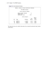
The estimates of the gamma distribution model, which is the best model according to a majority of the
EDF-based statistics, are shown in Figure 22.16. The estimate that is reported for the parameter Theta
is the base value for the scale parameter
Â
. If the gamma distribution is chosen to model
Y
, then the
effective value of the scale parameter is
 D 0:14293 exp.0:64562 x
1
 0:89831 x
2
C 0:14901 x
3
/
.
Syntax: SEVERITY Procedure ✦ 1509
Figure 22.16 Parameter Estimates for the Gamma Model with Regressors
Parameter Estimates for Gamma Distribution
Standard Approx
Parameter Estimate Error t Value Pr > |t|

Theta 0.14293 0.02329 6.14 <.0001
Alpha 20.37726 2.93277 6.95 <.0001
x1 0.64562 0.08224 7.85 <.0001
x2 -0.89831 0.07962 -11.28 <.0001
x3 0.14901 0.07870 1.89 0.0613
Syntax: SEVERITY Procedure
The following statements are used with the SEVERITY procedure.
PROC SEVERITY options ;
BY variable-list ;
MODEL response-variable < ( options ) > < = regressor-variable-list > < / fit-options > ;
DIST distribution-name <( distribution-options )> ;
NLOPTIONS options ;
Functional Summary
Table 22.1 summarizes the statements and options that control the SEVERITY procedure.
Table 22.1 SEVERITY Functional Summary
Description Statement Option
Statements
Specifies BY-group processing BY
Specifies the variables to model MODEL
Specifies a model to fit DIST
Specifies optimization options NLOPTIONS
Data Set Options
Specifies the input data set PROC SEVERITY DATA=
Specifies the output data set for parameter esti-
mates
PROC SEVERITY OUTEST=
Specifies that the OUTEST= data set contain
covariance estimates
PROC SEVERITY COVOUT
Specifies the output data set for statistics of fit PROC SEVERITY OUTSTAT=

1510 ✦ Chapter 22: The SEVERITY Procedure (Experimental)
Table 22.1 continued
Description Statement Option
Specifies the output data set for CDF estimates
PROC SEVERITY OUTCDF=
Specifies the output data set for model informa-
tion
PROC SEVERITY OUTMODELINFO=
Specifies the input data set for parameter esti-
mates
PROC SEVERITY INEST=
Data Interpretation Options
Specifies right-censoring MODEL RIGHTCENSORED=
Specifies left-truncation MODEL LEFTTRUNCATED=
Specifies the probability of observability MODEL PROBOBSERVED=
Model Estimation Options
Specifies the model selection criterion MODEL CRITERION=
Specifies initial values for model parameters DIST INIT=
Specifies the denominator for computing co-
variance estimates
PROC SEVERITY VARDEF=
Nonparametric CDF Estimation Options
Specifies the nonparametric method of CDF
estimation
MODEL EMPIRICALCDF=
Specifies the absolute lower bound on risk set
size when
EMPIRICALCDF=MODIFIEDKM
is specified
MODEL RSLB=

Specifies the
c
value for the
lower bound on risk set size when
EMPIRICALCDF=MODIFIEDKM
is speci-
fied
MODEL C=
Specifies the
˛
value for the
lower bound on risk set size when
EMPIRICALCDF=MODIFIEDKM
is speci-
fied
MODEL ALPHA=
Displayed Output and Plotting Options
Specifies that all displayed and graphical output
be turned off
PROC SEVERITY NOPRINT
Specifies the output to be displayed PROC SEVERITY PRINT=
Specifies that only the specified output be dis-
played
PROC SEVERITY ONLY
Specifies the graphical output to be displayed PROC SEVERITY PLOTS=
Specifies that only the specified plots be pre-
pared
PROC SEVERITY ONLY
Specifies that censored observations be marked
in appropriate plots

PROC SEVERITY MARKCENSORED
Specifies that truncated observations be marked
in appropriate plots
PROC SEVERITY MARKTRUNCATED
PROC SEVERITY Statement ✦ 1511
Table 22.1 continued
Description Statement Option
Specifies that histogram estimates be included
in PDF plots
PROC SEVERITY HISTOGRAM
Specifies that kernel estimates be included in
PDF plots
PROC SEVERITY KERNEL
PROC SEVERITY Statement
PROC SEVERITY options ;
The following options can be used in the PROC SEVERITY statement:
DATA=SAS-data-set
names the input data set. If the DATA= option is not specified, then the most recently created
SAS data set is used.
OUTEST=SAS-data-set
names the output data set to contain estimates of the parameter values and their standard errors
for each model whose parameter estimation process converges. Details of the variables in this
data set are provided in the section “OUTEST= Data Set” on page 1553.
COVOUT
specifies that the OUTEST= data set contain the estimate of the covariance structure of the
parameters. This option has no effect if the OUTEST= option is not specified. Details of how
the covariance is reported in OUTEST= data set are provided in the section “OUTEST= Data
Set” on page 1553.
VARDEF=option
specifies the denominator to use for computing the covariance estimates. The following options

are available:
DF
specifies that the number of nonmissing observations minus the model
degrees of freedom (number of parameters) be used.
N specifies that the number of nonmissing observations be used.
The details of the covariance estimation are provided in the section “Estimating Covariance
and Standard Errors” on page 1542.
OUTSTAT=SAS-data-set
names the output data set to contain the values of statistics of fit for each model whose
parameter estimation process converges. Details of the variables in this data set are provided
in the section “OUTSTAT= Data Set” on page 1554.