1272 ✦ Chapter 18: The MODEL Procedure
starts = (1 - d)
*
y1 + d
*
y2;
/
*
Resulting log-likelihood function
*
/
logL = (1/2)
*
( (log(2
*
3.1415)) +
log( (sig1
**
2)
*
((1-d)
**
2)+(sig2
**
2)
*
(d
**
2) )
+ (resid.starts
*

( 1/( (sig1
**
2)
*
((1-d)
**
2)+
(sig2
**
2)
*
(d
**
2) ) )
*
resid.starts) ) ;
errormodel starts ~ general(logL);
fit starts / method=marquardt converge=1.0e-5;
/
*
Test for significant differences in the parms
*
/
test int1 = int2 ,/ lm;
test b11 = b21 ,/ lm;
test b13 = b23 ,/ lm;
test sig1 = sig2 ,/ lm;
run;
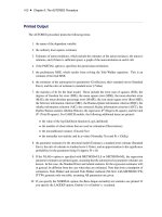
Four TEST statements are added to test the hypothesis that the parameters are the same in both
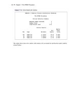
regimes. The parameter estimates and ANOVA table from this run are shown in Output 18.13.1.

Output 18.13.1 Parameter Estimates from the Switching Regression
Switching Regression Example
The MODEL Procedure
Nonlinear Liklhood Summary of Residual Errors
DF DF Adj
Equation Model Error SSE MSE R-Square R-Sq
starts 9 304 85878.0 282.5 0.7806 0.7748
Nonlinear Liklhood Parameter Estimates
Approx Approx
Parameter Estimate Std Err t Value Pr > |t|
sig1 15.47484 0.9476 16.33 <.0001
sig2 19.77808 1.2710 15.56 <.0001
int1 32.82221 5.9083 5.56 <.0001
b11 0.73952 0.0444 16.64 <.0001
b13 -15.4556 3.1912 -4.84 <.0001
int2 42.73348 6.8159 6.27 <.0001
b21 0.734117 0.0478 15.37 <.0001
b23 -22.5184 4.2985 -5.24 <.0001
p 25.94712 8.5205 3.05 0.0025
The test results shown in Output 18.13.2 suggest that the variance of the housing starts, SIG1 and
SIG2, are significantly different in the two regimes. The tests also show a significant difference in
the AR term on the housing starts.
Example 18.14: Simulating from a Mixture of Distributions ✦ 1273
Output 18.13.2 Test Results for Switching Regression
Test Results
Test Type Statistic Pr > ChiSq Label
Test0 L.M. 1.00 0.3185 int1 = int2
Test1 L.M. 15636 <.0001 b11 = b21
Test2 L.M. 1.45 0.2280 b13 = b23
Test3 L.M. 4.39 0.0361 sig1 = sig2

Example 18.14: Simulating from a Mixture of Distributions
This example illustrates how to perform a multivariate simulation by using models that have different
error distributions. Three models are used. The first model has t distributed errors. The second model
is a GARCH(1,1) model with normally distributed errors. The third model has a noncentral Cauchy
distribution.
The following SAS statements generate the data for this example. The t and the CAUCHY data sets
use a common seed so that those two series are correlated.
/
*
set distribution parameters
*
/
%let df = 7.5;
%let sig1 = .5;
%let var2 = 2.5;
data t;
format date monyy.;
do date='1jun2001'd to '1nov2002'd;
/
*
t-distribution with df,sig1
*
/
t = .05
*
date + 5000 + &sig1
*
tinv(ranuni(1234),&df);
output;
end;

run;
data normal;
format date monyy.;
le = &var2;
lv = &var2;
do date='1jun2001'd to '1nov2002'd;
/
*
Normal with GARCH error structure
*
/
v = 0.0001 + 0.2
*
le
**
2 + .75
*
lv;
e = sqrt( v)
*
rannor(12345) ;
normal = 25 + e;
le = e;
lv = v;
output;
end;
run;
1274 ✦ Chapter 18: The MODEL Procedure
data cauchy;
format date monyy.;

PI = 3.1415926;
do date='1jun2001'd to '1nov2002'd;
cauchy = -4 + tan((ranuni(1234) - 0.5)
*
PI);
output;
end;
run;
Since the multivariate joint likelihood is unknown, the models must be estimated separately. The
residuals for each model are saved by using the OUT= option. Also, each model is saved by using
the OUTMODEL= option. The ID statement is used to provide a variable in the residual data set
to merge by. The XLAG function is used to model the GARCH(1,1) process. The XLAG function
returns the lag of the first argument if it is nonmissing, otherwise it returns the second argument.
title1 't-distributed Errors Example';
proc model data=t outmod=tModel;
parms df 10 vt 4;
t = a
*
date + c;
errormodel t ~ t( vt, df );
fit t / out=tresid;
id date;
run;
title1 'GARCH-distributed Errors Example';
proc model data=normal outmodel=normalModel;
normal = b0 ;
h.normal = arch0 + arch1
*
xlag(resid.normal
**

2 , mse.normal)
+ GARCH1
*
xlag(h.normal, mse.normal);
fit normal /fiml out=nresid;
id date;
run;
title1 'Cauchy-distributed Errors Example';
proc model data=cauchy outmod=cauchyModel;
parms nc = 1;
/
*
nc is noncentrality parm to Cauchy dist
*
/
cauchy = nc;
obj = log(1+resid.cauchy
**
2
*
3.1415926);
errormodel cauchy ~ general(obj) cdf=cauchy(nc);
fit cauchy / out=cresid;
id date;
run;
Example 18.14: Simulating from a Mixture of Distributions ✦ 1275
The simulation requires a covariance matrix created from normal residuals. The following DATA
step statements use the inverse CDFs of the t and Cauchy distributions to convert the residuals to
the normal distribution. The CORR procedure is used to create a correlation matrix that uses the
converted residuals.

/
*
Merge and normalize the 3 residual data sets
*
/
data c; merge tresid nresid cresid; by date;
t = probit(cdf("T", t/sqrt(0.2789), 16.58 ));
cauchy = probit(cdf("CAUCHY", cauchy, -4.0623));
run;
proc corr data=c out=s;
var t normal cauchy;
run;
Now the models can be simulated together by using the MODEL procedure SOLVE statement. The
data set created by the CORR procedure is used as the correlation matrix.
title1 'Simulating Equations with Different Error Distributions';
/
*
Create one observation driver data set
*
/
data sim; merge t normal cauchy; by date;
data sim; set sim(firstobs = 519 );
proc model data=sim model=( tModel normalModel cauchyModel );
errormodel t ~ t( vt, df );
errormodel cauchy ~ cauchy(nc);
solve t cauchy normal / random=2000 seed=1962 out=monte
sdata=s(where=(_type_="CORR"));
run;
An estimation of the joint density of the t and Cauchy distribution is created by using the KDE
procedure. Bounds are placed on the Cauchy dimension because of its fat tail behavior. The joint

PDF is shown in Output 18.14.1.
title "T and Cauchy Distribution";
proc kde data=monte;
univar t / out=t_dens;
univar cauchy / out=cauchy_dens;
bivar t cauchy / out=density
plots=all;
run;
1276 ✦ Chapter 18: The MODEL Procedure
Output 18.14.1 Bivariate Density of t and Cauchy, Distribution of t by Cauchy
Example 18.14: Simulating from a Mixture of Distributions ✦ 1277
Output 18.14.2 Bivariate Density of t and Cauchy, Kernel Density for t and Cauchy
1278 ✦ Chapter 18: The MODEL Procedure
Output 18.14.3 Bivariate Density of t and Cauchy, Distribution and Kernel Density for t and
Cauchy
Example 18.14: Simulating from a Mixture of Distributions ✦ 1279
Output 18.14.4 Bivariate Density of t and Cauchy, Distribution of t by Cauchy
1280 ✦ Chapter 18: The MODEL Procedure
Output 18.14.5 Bivariate Density of t and Cauchy, Kernel Density for t and Cauchy
Example 18.15: Simulated Method of Moments—Simple Linear Regression ✦ 1281
Output 18.14.6 Bivariate Density of t and Cauchy, Distribution and Kernel Density for t and
Cauchy
Example 18.15: Simulated Method of Moments—Simple Linear
Regression
This example illustrates how to use SMM to estimate a simple linear regression model for the
following process:
y D a Cbx C ;   i id N.0; s
2
/
In the following SAS statements,

ysim
is simulated, and the first moment and the second moment of
ysim are compared with those of the observed endogenous variable y.
title "Simple regression model";
data regdata;