626 LINEAR PARTIAL DIFFERENTIAL EQUATIONS
14.8.3. Problems for Equation
∂
2
w
∂t
2
+ a(t)
∂w
∂t
= b(t)

∂
∂x

p(x)
∂w
∂x

– q(x)w

+ Φ(x, t)
14.8.3-1. General relations to solve nonhomogeneous boundary value problems.
Consider the generalized telegraph equation of the form
∂
2
w
∂t
2
+ a(t)
∂w

∂t
= b(t)

∂
∂x

p(x)
∂w
∂x

– q(x)w

+ Φ(x, t). (14.8.3.1)
It is assumed that the functions p, p

x
,andq are continuous and p > 0 for x
1
≤ x ≤ x
2
.
The solution of equation (14.8.3.1) under the general initial conditions (14.8.1.2) and
the arbitrary linear nonhomogeneous boundary conditions (14.8.1.3)–(14.8.1.4) can be
represented as the sum
w(x, t)=

t
0

x

2
x
1
Φ(ξ, τ)G(x, ξ, t, τ ) dξ dτ
–

x
2
x
1
f
0
(ξ)

∂
∂τ
G(x, ξ, t, τ )

τ=0
dξ +

x
2
x
1

f
1
(ξ)+a(0)f
0

(ξ)

G(x, ξ, t, 0) dξ
+ p(x
1
)

t
0
g
1
(τ)b(τ)Λ
1
(x, t, τ) dτ + p(x
2
)

t
0
g
2
(τ)b(τ)Λ
2
(x, t, τ) dτ .(14.8.3.2)
Here, the modified Green’s function is determined by
G(x, ξ, t, τ )=
∞

n=1
y

n
(x)y
n
(ξ)
y
n

2
U
n
(t, τ ), y
n

2
=

x
2
x
1
y
2
n
(x) dx,(14.8.3.3)
where the λ
n
and y
n
(x) are the eigenvalues and corresponding eigenfunctions of the Sturm–
Liouville problem for the following second-order linear ordinary differential equation with

homogeneous boundary conditions:
[p(x)y

x
]

x
+[λ – q(x)]y = 0,
α
1
y

x
+ β
1
y = 0 at x = x
1
,
α
2
y

x
+ β
2
y = 0 at x = x
2
.
(14.8.3.4)
The functions U

n
= U
n
(t, τ ) are determined by solving the Cauchy problem for the linear
ordinary differential equation
U

n
+ a(t)U

n
+ λ
n
b(t)U
n
= 0,
U
n


t=τ
= 0, U

n


t=τ
= 1.
(14.8.3.5)
The prime denotes the derivative with respect to t,andτ is a free parameter occurring in

the initial conditions.
The functions Λ
1
(x, t)andΛ
2
(x, t) that occur in the integrands of the last two terms
in solution (14.8.3.2) are expressed in terms of the Green’s function of (14.8.3.3). The
corresponding formulas will be specified below when studying specific boundary value
problems.
The general and special properties of the Sturm–Liouville problem (14.8.3.4) are de-
tailed in Subsection 12.2.5. Asymptotic and approximate formulas for eigenvalues and
eigenfunctions are also presented there.
14.8. BOUNDARY VALUE PROBLEMS FOR HYPERBOLIC EQUATIONS WITH ONE SPACE VARIABLE 627
14.8.3-2. First, second, third, and mixed boundary value problems.
1
◦
. First boundary value problem. The solution of equation (14.8.3.1) with the initial
conditions (14.8.1.2) and boundary conditions (14.8.1.3)–(14.8.1.4) for α
1
= α
2
= 0 and
β
1
= β
2
= 1 is given by relations (14.8.3.2) and (14.8.3.3), where
Λ
1
(x, t, τ)=

∂
∂ξ
G(x, ξ, t, τ )



ξ=x
1
, Λ
2
(x, t, τ)=–
∂
∂ξ
G(x, ξ, t, τ )



ξ=x
2
.
2
◦
. Second boundary value problem. The solution of equation (14.8.3.1) with the initial
conditions (14.8.1.2) and boundary conditions (14.8.1.3)–(14.8.1.4) for α
1
= α
2
= 1 and
β
1

= β
2
= 0 is given by relations (14.8.3.2) and (14.8.3.3) with
Λ
1
(x, t, τ)=–G(x, x
1
, t, τ ), Λ
2
(x, t, τ)=G(x, x
2
, t, τ ).
3
◦
. Third boundary value problem. The solution of equation (14.8.3.1) with the initial
conditions (14.8.1.2) and boundary conditions (14.8.1.3)–(14.8.1.4) for α
1
= α
2
= 1 and
β
1
β
2
≠ 0 is given by relations (14.8.3.2) and (14.8.3.3) in which
Λ
1
(x, t, τ)=–G(x, x
1
, t, τ ), Λ

2
(x, t, τ)=G(x, x
2
, t, τ ).
4
◦
. Mixed boundary value problem. The solution of equation (14.8.3.1) with the initial
conditions (14.8.1.2) and boundary conditions (14.8.1.3)–(14.8.1.4) for α
1
= β
2
= 0 and
α
2
= β
1
= 1 is given by relations (14.8.3.2) and (14.8.3.3) with
Λ
1
(x, t, τ)=
∂
∂ξ
G(x, ξ, t, τ )



ξ=x
1
, Λ
2

(x, t, τ)=G(x, x
2
, t, τ ).
5
◦
. Mixed boundary value problem. The solution of equation (14.8.3.1) with the initial
conditions (14.8.1.2) and boundary conditions (14.8.1.3)–(14.8.1.4) for α
1
= β
2
= 1 and
α
2
= β
1
= 0 is given by relations (14.8.3.2) and (14.8.3.3) with
Λ
1
(x, t, τ)=–G(x, x
1
, t, τ ), Λ
2
(x, t, τ)=–
∂
∂ξ
G(x, ξ, t, τ )



ξ=x

2
.
14.8.4. Generalized Cauchy Problem with Initial Conditions Set
Along a Curve
14.8.4-1. Statement of the generalized Cauchy problem. Basic property of a solution.
Consider the general linear hyperbolic equation in two independent variables which is
reduced to the first canonical form (see Paragraph 14.1.1-4):
∂
2
w
∂x∂y
+ a(x, y)
∂w
∂x
+ b(x, y)
∂w
∂y
+ c(x, y)w = f (x, y), (14.8.4.1)
where a(x, y), b(x, y), c(x, y), and f (x, y) are continuous functions.
Let a segment of a curve in the xy-plane be defined by
y = ϕ(x)(α ≤ x ≤ β), (14.8.4.2)
where ϕ(x) is continuously differentiable, with ϕ

(x) ≠ 0 and ϕ

(x) ≠ ∞.
628 LINEAR PARTIAL DIFFERENTIAL EQUATIONS
The generalized Cauchy problem for equation (14.8.4.1) with initial conditions defined
along a curve (14.8.4.2) is stated as follows: find a solution to equation (14.8.4.1) that
satisfies the conditions

w(x, y)|
y=ϕ(x)
= g(x),
∂w
∂x



y=ϕ(x)
= h
1
(x),
∂w
∂y



y=ϕ(x)
= h
2
(x), (14.8.4.3)
where g(x), h
1
(x), and h
2
(x) are given continuous functions, related by the compatibility
condition
g

x

(x)=h
1
(x)+h
2
(x)ϕ

x
(x). (14.8.4.4)
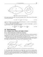
Basic property of the generalized Cauchy problem: the value of the solution at any point
M(x
0
, y
0
) depends only on the values of the functions g(x), h
1
(x), and h
2
(x)onthearc
AB, cut off on the given curve (14.8.4.2) by the characteristics x = x
0
and y = y
0
,and
on the values of a(x, y), b(x, y), c(x, y), and f(x, y) in the curvilinear triangle AM B;see
Fig. 14.3. The domain of influence on the solution at M(x
0
, y
0
) is shaded for clarity.
characteristics

B
A
y= xφ()
y
x
x
y
0
0
O
Mx y(, )
00
Figure 14.3. Domain of influence of the solution to the generalized Cauchy problem at a point M.
Remark 1. Rather than setting two derivatives in the boundary conditions (14.8.4.3), it suffices to set
either of them, with the other being uniquely determined from the compatibility condition (14.8.4.4).
Remark 2. Instead of the last two boundary conditions in (14.8.4.3), the value of the derivative along the
normal to the curve (14.8.4.2) can be used:
∂w
∂n



y=ϕ(x)
≡
1

1 +[ϕ

x
(x)]

2

∂w
∂y
– ϕ

x
(x)
∂w
∂x

y=ϕ(x)
= h
3
(x). (14.8.4.5)
Denoting w
x
|
y=ϕ(x)
= h
1
(x)andw
y
|
y=ϕ(x)
= h
2
(x), we have
h
2

(x)–ϕ

x
(x)h
1
(x)=h
3
(x)

1 +[ϕ

x
(x)]
2
.(14.8.4.6)
The functions h
1
(x)andh
2
(x) can be found from (14.8.4.4) and (14.8.4.6). Further substituting their expres-
sions into (14.8.4.3), one arrives at the standard formulation of the generalized Cauchy problem, where the
compatibility condition for initial data (14.8.4.4) will be satisfied automatically.
14.8.4-2. Riemann function.
A Riemann function, R = R(x, y; x
0
, y
0
), corresponding to equation (14.8.4.1) is defined
as a solution to the equation
∂

2
R
∂x∂y
–
∂
∂x

a(x, y)R

–
∂
∂y

b(x, y)R

+ c(x, y)R = 0 (14.8.4.7)
14.8. BOUNDARY VALUE PROBLEMS FOR HYPERBOLIC EQUATIONS WITH ONE SPACE VARIABLE 629
that satisfies the conditions
R =exp


y
y
0
a(x
0
, ξ) dξ

at x = x
0

, R =exp


x
x
0
b(ξ, y
0
) dξ

at y = y
0
(14.8.4.8)
at the characteristics x = x
0
and y = y
0
. Here, (x
0
, y
0
) is an arbitrary point from the domain
of equation (14.8.4.1). The x
0
and y
0
appear in problem (14.8.4.7)–(14.8.4.8) as parameters
in the boundary conditions only.
T
HEOREM.

If the functions
a
,
b
,
c
and the partial derivatives
a
x
,
b
y
are all continuous,
then the Riemann function
R(x, y;x
0
, y
0
)
exists. Moreover, the function
R(x
0
, y
0
, x, y)
,
obtained by swapping the parameters and the arguments, is a solution to the homogeneous
equation (14.8.4.1), with
f = 0
.

Remark. It is significant that the Riemann function depends on neither the shape of the curve (14.8.4.2)
nor the initial data set on it (14.8.4.3).
Example 1. The Riemann function for the equation w
xy
= 0 is just R ≡ 1.
Example 2. The Riemann function for the equation
w
xy
+ cw = 0 (c = const) (14.8.4.9)
is expressed via the Bessel function J
0
(z)as
R = J
0


4c(x
0
– x)(y
0
– y)

.
Remark. Any linear constant-coefficient partial differential equation of the parabolic type in two inde-
pendent variables can be reduced to an equation of the form (14.8.4.9); see Paragraph 14.1.1-6.
14.8.4-3. Solution of the generalized Cauchy problem via the Riemann function.
Given a Riemann function, the solution to the generalized Cauchy problem (14.8.4.1)–
(14.8.4.3) at any point (x
0
, y

0
) can written as
w(x
0
, y
0
)=
1
2
(wR)
A
+
1
2
(wR)
B
+
1
2

AB

R
∂w
∂x
– w
∂R
∂x
+ 2bwR


dx
–
1
2

AB

R
∂w
∂y
– w
∂R
∂y
+ 2awR

dy +

ΔAMB
fRdx dy.
The first two terms on the right-hand side are evaluated as the points A and B. The third
and fourth terms are curvilinear integrals over the arc AB;thearcisdefined by equation
(14.8.4.2), and the integrands involve quantities defined by the initial conditions (14.8.4.3).
The last integral is taken over the curvilinear triangular domain AMB.
14.8.5. Goursat Problem (a Problem with Initial Data of
Characteristics)
14.8.5-1. Statement of the Goursat problem. Basic property of the solution.
The Goursat problem for equation (14.8.4.1) is stated as follows: find a solution to equation
(14.8.4.1) that satisfies the conditions at characteristics
w(x, y)|
x=x

1
= g(y), w(x, y)|
y=y
1
= h(x), (14.8.5.1)
630 LINEAR PARTIAL DIFFERENTIAL EQUATIONS
where g(y)andh(x) are given continuous functions that match each other at the point of
intersection of the characteristics, so that
g(y
1
)=h(x
1
).
Basic properties of the Goursat problem: the value of the solution at any point M(x
0
, y
0
)
depends only on the values of g(y) at the segment AN (which is part of the characteristic
x = x
1
), the values of h(x) at the segment BN (which is part of the characteristic y = y
1
),
and the values of the functions a(x, y), b(x, y), c(x, y), and f(x, y) in the rectangle NAMB;
see Fig. 14.4. The domain of influence on the solution at the point M(x
0
, y
0
) is shaded for

clarity.
Nx y(, )
characteristics
B
A
y
x
xx
y
y=y
x=x
y
01
1
Mx y(, )
00
1
0
1
1
1
O
Figure 14.4. Domain of influence of the solution to the Goursat problem at a point M .
14.8.5-2. Solution representation for the Goursat problem via the Riemann function.
Given a Riemann function (see Paragraph 14.8.4-2), the solution to the Goursat problem
(14.8.4.1), (14.8.5.1) at any point (x
0
, y
0
) can be written as

w(x
0
, y
0
)=(wR)
N
+

A
N
R

g

y
+ bg

dy +

B
N
R

h

x
+ ah

dx +


NAMB
fRdx dy.
The first term on the right-hand side is evaluated at the point of intersection of the charac-
teristics (x
1
, y
1
). The second and third terms are integrals along the characteristics y = y
1
(x
1
≤ x ≤ x
0
)andx = x
1
(y
1
≤ y ≤ y
0
); these involve the initial data of (14.8.5.1). The last in-
tegral is taken over the rectangular domain NAMBdefined by the inequalities x
1
≤ x ≤ x
0
,
y
1
≤ y ≤ y
0
.

The Goursat problem for hyperbolic equations reduced to the second canonical form
(see Paragraph 14.1.1-4) is treated similarly.
Example. Consider the Goursat problem for the wave equation
∂
2
w
∂t
2
– a
2
∂
2
w
∂x
2
= 0
with the boundary conditions prescribed on its characteristics
w = f(x)forx – at = 0 (0 ≤ x ≤ b),
w = g(x)forx + at = 0 (0 ≤ x ≤ c),
(14.8.5.2)
where f(0)=g(0).
Substituting the values set on the characteristics (14.8.5.2) into the general solution of the wave equation,
w = ϕ(x – at)+ψ(x + at), we arrive to a system of linear algebraic equations for ϕ(x)andψ(x). As a result,
the solution to the Goursat problem is obtained in the form
w(x, t)=f

x + at
2

+ g


x – at
2

– f(0).
The solution propagation domain is the parallelogram bounded by the four lines
x – at = 0, x + at = 0, x – at = 2c, x + at = 2b.
14.9. BOUNDARY VALUE PROBLEMS FOR ELLIPTIC EQUATIONS WITH TWO SPACE VARIABLES 631
14.9. Boundary Value Problems for Elliptic Equations
with Two Space Variables
14.9.1. Problems and the Green’s Functions for Equation
a(x)
∂
2
w
∂x
2
+
∂
2
w
∂y
2
+ b(x)
∂w
∂x
+ c(x)w =–Φ(x, y)
14.9.1-1. Statements of boundary value problems.
Consider two-dimensional boundary value problems for the equation
a(x)

∂
2
w
∂x
2
+
∂
2
w
∂y
2
+ b(x)
∂w
∂x
+ c(x)w =–Φ(x, y)(14.9.1.1)
with general boundary conditions in x,
α
1
∂w
∂x
– β
1
w = f
1
(y)atx = x
1
,
α
2
∂w

∂x
+ β
2
w = f
2
(y)atx = x
2
,
(14.9.1.2)
and different boundary conditions in y. Itisassumedthatthecoefficients of equation
(14.9.1.1) and the boundary conditions (14.9.1.2) meet the requirements
a(x), b(x), c(x) are continuous (x
1
≤ x ≤ x
2
); a > 0, |α
1
| + |β
1
| > 0, |α
2
| + |β
2
| > 0.
14.9.1-2. Relations for the Green’s function.
In the general case, the Green’s function can be represented as
G(x, y, ξ, η)=ρ(ξ)
∞

n=1

u
n
(x)u
n
(ξ)
u
n

2
Ψ
n
(y, η; λ
n
). (14.9.1.3)
Here,
ρ(x)=
1
a(x)
exp


b(x)
a(x)
dx

, u
n

2
=


x
2
x
1
ρ(x)u
2
n
(x) dx,(14.9.1.4)
and the λ
n
and u
n
(x) are the eigenvalues and eigenfunctions of the homogeneous boundary
value problem for the ordinary differential equation
a(x)u

xx
+ b(x)u

x
+[λ + c(x)]u = 0,(14.9.1.5)
α
1
u

x
– β
1
u = 0 at x = x

1
,(14.9.1.6)
α
2
u

x
+ β
2
u = 0 at x = x
2
.(14.9.1.7)
The functions Ψ
n
for various boundary conditions in y are specified in Table 14.8.
Equation (14.9.1.5) can be rewritten in self-adjoint form as
[p(x)u

x
]

x
+[λρ(x)–q(x)]u = 0,(14.9.1.8)
632 LINEAR PARTIAL DIFFERENTIAL EQUATIONS
TABLE 14.8
The functions Ψ
n
in (14.9.1.3) for various boundary conditions.* Notation: σ
n
=

√
λ
n
Domain Boundary conditions Function Ψ
n
(y, η; λ
n
)
–∞ < y < ∞
|w| < ∞ for y → ∞
1
2σ
n
e
–σ
n
|y–η|
0 ≤ y < ∞ w = 0 for y = 0
1
σ
n

e
–σ
n
y
sinh(σ
n
η)fory > η,
e

–σ
n
η
sinh(σ
n
y)forη > y
0 ≤ y < ∞
∂
y
w = 0 for y = 0
1
σ
n

e
–σ
n
y
cosh(σ
n
η)fory > η,
e
–σ
n
η
cosh(σ
n
y)forη > y
0 ≤ y < ∞
∂

y
w – β
3
w = 0 for y = 0
1
σ
n
(σ
n
+ β
3
)

e
–σ
n
y
[σ
n
cosh(σ
n
η)+β
3
sinh(σ
n
η)] for y > η,
e
–σ
n
η

[σ
n
cosh(σ
n
y)+β
3
sinh(σ
n
y)] for η > y
0 ≤ y ≤ h
w = 0 at y = 0,
w = 0 at y = h
1
σ
n
sinh(σ
n
h)

sinh(σ
n
η)sinh[σ
n
(h – y)] for y > η,
sinh(σ
n
y)sinh[σ
n
(h – η)] for η > y
0 ≤ y ≤ h

∂
y
w = 0 at y = 0,
∂
y
w = 0 at y = h
1
σ
n
sinh(σ
n
h)

cosh(σ
n
η)cosh[σ
n
(h – y)] for y > η,
cosh(σ
n
y)cosh[σ
n
(h – η)] for η > y
0 ≤ y ≤ h
w = 0 at y = 0,
∂
y
w = 0 at y = h
1
σ

n
cosh(σ
n
h)

sinh(σ
n
η)cosh[σ
n
(h – y)] for y > η,
sinh(σ
n
y)cosh[σ
n
(h – η)] for η > y
where the functions p(x)andq(x)aregivenby
p(x)=exp


b(x)
a(x)
dx

, q(x)=–
c(x)
a(x)
exp


b(x)

a(x)
dx

,
and ρ(x)isdefined in (14.9.1.4).
The eigenvalue problem (14.9.1.8), (14.9.1.6), (14.9.1.7) possesses the following prop-
erties:
1
◦
. All eigenvalues λ
1
, λ
2
, are real and λ
n
→∞as n →∞.
2
◦
. Thesystem of eigenfunctions {u
1
(x), u
2
(x), } is orthogonal on the intervalx
1
≤x≤x
2
with weight ρ(x), that is,

x
2

x
1
ρ(x)u
n
(x)u
m
(x) dx = 0 for n ≠ m.
3
◦
. If the conditions
q(x) ≥ 0, α
1
β
1
≥ 0, α
2
β
2
≥ 0 (14.9.1.9)
are satisfied, there are no negative eigenvalues. If q ≡ 0 and β
1
= β
2
= 0, then the least
eigenvalue is λ
0
= 0 and the corresponding eigenfunction is u
0
= const; in this case, the
summation in (14.9.1.3) must start with n = 0. In the other cases, if conditions (14.9.1.9)

are satisfied, all eigenvalues are positive; for example, the first inequality in (14.9.1.9) holds
if c(x) ≤ 0.
Subsection 12.2.5 presents some relations for estimating the eigenvalues λ
n
and eigen-
functions u
n
(x).
* For unbounded domains, the condition of boundedness of the solution as y → ∞ is set; in Table 14.8,
this condition is omitted.