1.2 Oscillations of Three Species; Atmospheric Neutrinos 21
later time t. Write the probability P
α→β
(t) to observe a neutrino of flavor β
at time t.
1.2.2. We define the oscillation lengths at an energy E  pc by:
L
ij
=
4π¯hp
|∆m
2
ij
|c
2
,∆m
2
ij
= m
2
i
− m
2
j
. (1.9)
Notice that there are only two independent oscillation lengths since ∆m
2
12
+
∆m
2

23
+ ∆m
2
31
= 0. For neutrinos of energy E = 4 GeV, calculate the oscilla-
tion lengths L
12
and L
23
. We will choose for |∆m
2
12
| the result given in (1.7),
and we will choose |∆m
2
23
|c
4
=2.5 ×10
−3
eV
2
, a value which will be justified
later on.
1.2.3. The neutrino counters have an accuracy of the order of 10% and the
energy is E = 4 GeV. Above which distances 
12
and 
23
of the production

point of the neutrinos can one hope to detect oscillations coming from the
superpositions 1 ↔ 2and2↔ 3?
1.2.4. The Super-Kamiokande experiment, performed in 1998, consists in de-
tecting “atmospheric” neutrinos. Such neutrinos are produced in the collision
of high energy cosmic rays with nuclei in the atmosphere at high altitudes.
In a series of reactions, π
±
mesons are produced abundantly, and they decay
through the chain:
π
−
→ µ
−
+¯ν
µ
followed by µ
−
→ e
−
+¯ν
e
+ ν
µ
, (1.10)
and an analogous chain for π
+
mesons. The neutrino fluxes are detected in
an underground detector by the reactions (1.1) and (1.3).
To simplify things, we assume that all muons decay before reaching the
surface of the Earth. Deduce that, in the absence of neutrino oscillations, the

expected ratio between electron and muon neutrinos
R
µ/e
=
N(ν
µ
)+N(¯ν
µ
)
N(ν
e
)+N(¯ν
e
)
would be equal to 2.
1.2.5. The corrections to the ratio R
µ/e
due to the fact that part of the
muons reach the ground can be calculated accurately. Once this correction is
made, one finds, by comparing the measured and calculated values for R
µ/e
(R
µ/e
)
measured
(R
µ/e
)
calculated
=0.64 (±0.05) .

In order to explain this relative decrease of the number of ν
µ
’s, one can think
of oscillations of the types ν
µ


ν
e
and ν
µ


ν
τ
. The Super-Kamiokande ex-
periment consists in varying the time of flight of the neutrinos by measuring
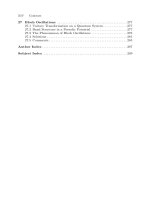
selectively the direction where they come from, as indicated on Fig. 1.2. The
22 1 Neutrino Oscillations
Earth
Detector
zenithal
angle α
atmosphere
cosmic
ray
neutrino
0
0,5-0,5-1 1
40

0
80
120
Electron neutrinos
cos α
0
0,5-0,5-1 1
0
200
300
100
Muon neutrinos
cos α
Fig. 1.2. Left: production of atmospheric neutrinos in collisions of cosmic rays
with terrestrial atmospheric nuclei. The underground detector measures the flux of
electron and muon neutrinos as a function of the zenithal angle α. Right: number
of atmospheric neutrinos detected in the Super-Kamiokande experiment as a func-
tion of the zenithal angle (this picture is drawn after K. Tanyaka, XXII Physics in
Collisions Conference, Stanford 2002)
neutrinos coming from above (cos α ∼ 1) have traveled a distance equal to the
atmospheric height plus the depth of the detector, while those coming from
the bottom (cos α ∼−1) have crossed the diameter of the Earth (13 400 km).
Given the weakness of the interaction of neutrinos with matter, one can con-
sider that the neutrinos propagate freely on a measurable distance between a
few tens of km and 13 400 km.
The neutrino energies are typically 4 GeV in this experiment. Can one
observe a ν
e



ν
µ
oscillation of the type studied in the first part?
1.2.6. The angular distributions of the ν
e
and the ν
µ
are represented on
Fig. 1.2, together with the distributions one would observe in the absence
of oscillations. Explain why this data is compatible with the fact that one
observes a ν
µ


ν
τ
oscillation, no ν
e


ν
τ
oscillation, and no ν
e


ν
µ
oscillation.
1.3 Solutions 23

1.2.7. In view of the above results, we assume that there is only a two-
neutrino oscillation phenomenon: ν
µ


ν
τ
in such an observation. We there-
fore use the same formalism as in the first part, except that we change the
names of particles.
By comparing the muon neutrino flux coming from above and from below,
give an estimate of the mixing angle θ
23
. In order to take into account the large
energy dispersion of cosmic rays, and therefore of atmospheric neutrinos, we
replace the oscillating factor sin
2
(π/L
23
) by its mean value 1/2if  L
23
.
The complete results published by the Super-Kamiokande experiment are
|∆m
2
23
|c
4
=2.5 × 10
−3

eV
2
,θ
23
= π/4 ,θ
13
=0.
Do they agree with the above considerations?
1.3 Solutions
Section 1.1: Mechanism of the Oscillations: Reactor Neutrinos
1.1.1. Initially, the neutrino state is |ν(0) = |ν
e
 = |ν
1
cos θ + |ν
2
sin θ.
Therefore, we have at time t
|ν(t) = |ν
1
 cos θ e
−iE
1
t/¯h
+ |ν
2
 sin θ e
−iE
2
t/¯h

.
1.1.2. The probability to find this neutrino in the state |ν
e
 at time t is
P
e
(t)=|ν
e
|ν(t)|
2
=



cos
2
θ e
−iE
1
t/¯h
+sin
2
θ e
−iE
2
t/¯h



2

,
which gives, after a simple calculation:
P
e
(t)=1− sin
2
(2θ)sin
2

(E
1
− E
2
)t
2¯h

.
We have E
1
− E
2
=(m
2
1
− m
2
2
)c
4
/(2pc). Defining the oscillation length by

L =4π¯hp/(|∆m
2
|c
2
), we obtain
P
e
(t)=1− sin
2
(2θ)sin
2

πct
L

.
1.1.3. For an energy E = pc =4MeVandamassdifference∆m
2
c
4
=
10
−4
eV
2
, we obtain an oscillation length L = 100 km.
1.1.4. The time of flight is t = /c. The probability P
e
() is therefore
P

e
()=1− sin
2
(2θ)sin
2

π
L

. (1.11)
24 1 Neutrino Oscillations
1.1.5. A ν
µ
energy of only 4 MeV is below the threshold of the reaction
ν
µ
+ n → p +µ. Therefore this reaction does not occur with reactor neutrinos,
and one cannot measure the ν
µ
flux.
1.1.6. In order to detect a significant decrease in the neutrino flux ν
e
,we
must have
sin
2
(2θ)sin
2

π

L

> 0.1 .
(a) For the maximum mixing θ = π/4, i.e. sin
2
(2θ) = 1, this implies π/L >
0.32 or >L/10. For E =4MeVand∆m
2
c
4
=10
−4
eV
2
, one finds >
10 km. The typical distances necessary to observe this phenomenon are of the
order of a fraction of the oscillation length.
(b) If the mixing is not maximum, one must operate at distances  greater
than L/10. Note that is the mixing angle is too small, (sin
2
(2θ) < 0.1 i.e.
θ<π/10), the oscillation amplitude is too weak to be detected, whatever the
distance . In that case, one must improve the detection efficiency to obtain
a positive conclusion.
1.1.7. (a) In all experiments except KamLAND, the distance is smaller
than 1 km. Therefore, in all of these experiments |1 − P
e
|≤10
−3
. The oscil-

lation effect is not detectable if the estimate |∆m
2
|c
4
∼ 10
−4
eV
2
is correct.
(b) For |∆m
2
|c
4
=7.1 ×10
−5
eV
2
,tan
2
θ =0.45 and  = 180 km, we obtain
P
e
=0.50 which agrees with the measurement. The theoretical prediction
taking into account the effects due to the dispersion in energy is drawn on
Fig. 1.3. We see incidentally how important it is to control error bars in such
an experiment.
ILL
Chooz
KamLAND
Bugey

Rovno
Goesgen
1,0
1,2
0,8
0,6
0,4
0,2
0
10
10
2
10
3
10
4
10
5
distance (meters)
N
detected
N
expected
Fig. 1.3. Experimental points of Fig. 1.1 and the theoretical prediction of (1.11)
(sinusoidal function damped by energy dispersion affects). This curve is a best fit of
solar neutrino data. We notice that the KamLAND data point corresponds to the
second oscillation of the curve
1.3 Solutions 25
Section 1.2: Oscillations of Three Species: Atmospheric Neutrinos
1.2.1. At time t =0,wehave:

|ν(0) = |ν
α
 =

j
U
αj
|ν
j
 ,
and therefore at time t:
|ν(t) =e
−ipct/¯h

j
U
αj
e
−im
2
j
c
3
t/(2¯hp)
|ν
j
 .
We conclude that the probability P
α→β
to observe a neutrino of flavor β at

time t is
P
α→β
(t)=|ν
β
|ν(t)|
2
=







j
U
∗
βj
U
αj
e
−im
2
j
c
3
t/(2¯hp)







2
.
1.2.2. We have L
ij
=4π¯hE/(|∆m
2
ij
|c
3
). The oscillation lengths are propor-
tional to the energy. We can use the result of question 1.3, with a conversion
factor of 1000 to go from 4 MeV to 4 GeV.
• For |∆m
2
12
|c
4
=7.1 × 10
−5
eV
2
, we find L
12
= 140 000 km.
• For |∆m
2

23
|c
4
=2.5 × 10
−3
eV
2
, we find L
23
= 4 000 km.
1.2.3. We want to know the minimal distance necessary in order to observe
oscillations. We assume that both mixing angles θ
12
and θ
23
are equal to
π/4, which corresponds to maximum mixing. We saw in the first part that if
this mixing is not maximum, the visibility of the oscillations is reduced and
that the distance which is necessary to observe the oscillation phenomenon is
increased.
By resuming the argument of the first part, we find that the modification of
the neutrino flux of a given species is detectable beyond a distance 
ij
such that
sin
2
(π
ij
/L
ij

) ≥ 0.1 i.e. 
ij
≥ L
ij
/10. This corresponds to 
12
≥ 14000 km for
the oscillation resulting from the superposition 1 ↔ 2, and 
23
≥ 400 km for
the oscillation resulting from the superposition 2 ↔ 3.
1.2.4. The factor of 2 between the expected muon and electron neutrino
fluxes comes from a simple counting. Each particle π
−
(resp. π
+
) gives rise to
a ν
µ
,a¯ν
µ
and a ¯ν
e
(resp. a ν
µ
,a¯ν
µ
and a ν
e
). In practice, part of the muons

reach the ground before decaying, which modifies this ratio. Naturally, this
effect is taken into account in an accurate treatment of the data.
1.2.5. For an energy of 4 GeV, we have found that the minimum distance to
observe the oscillation resulting from the 1 ↔ 2 superposition is 14000 km. We
therefore remark that the oscillations ν
e


ν
µ
, corresponding to the mixing
1 ↔ 2 which we studied in the first part cannot be observed at terrestrial
distances. At such energies (4 GeV) and for evolution times corresponding at
26 1 Neutrino Oscillations
most to the diameter of the Earth (0.04 s), the energy difference E
1
−E
2
and
the oscillations that it induces can be neglected.
However, if the estimate |∆m
2
23
|c
4
> 10
−3
eV
2
is correct, the terrestrial

distance scales allow in principle to observe oscillations resulting from 2 ↔ 3
and 1 ↔ 3 superpositions, which correspond to ν
µ


ν
τ
or ν
e


ν
τ
.
1.2.6. The angular distribution (therefore the distribution in ) observed for
the ν
e
’s does not show any deviation from the prediction made without any
oscillation. However, there is a clear indication for ν
µ
oscillations: there is a
deficit of muon neutrinos coming from below, i.e. those which have had a long
time to evolve.
The deficit in muon neutrinos is not due to the oscillation ν
e


ν
µ
of the

first part. Indeed, we have seen in the previous question that this oscillation is
negligible at time scales of interest. The experimental data of Fig. 1.2 confirm
this observation. The deficit in muon neutrinos coming from below is not
accompanied with an increase of electron neutrinos. The effect can only be
due to a ν
µ


ν
τ
oscillation.
1
No oscillation ν
e


ν
τ
appears in the data. In the framework of the present
model, this is interpreted as the signature of a very small (if not zero) θ
13
mixing angle.
1.2.7. Going back to the probability (1.11) written in question 1.4, the prob-
ability for an atmospheric muon neutrino ν
µ
to be detected as a ν
µ
is:
P ()=1− sin
2

(2θ
23
) sin
2

π
L
23

, (1.12)
where the averaging is performed on the energy distribution of the neutrino.
If we measure the neutrino flux coming from the top, we have   L
23
,which
gives P
top
= 1. If the neutrino comes from the bottom, the term sin
2
(π/L
23
)
averages to 1/2 and we find:
P
bottom
=1−
1
2
sin
2
(2θ

23
) .
The experimental data indicate that for −1 ≤ cos α ≤−0.5, P
bottom
=1/2.
The distribution is very flat at a value of 100 events, i.e. half of the top value
(200 events).
We deduce that sin
2
(2θ
23
) = 1, i.e. θ
23
= π/4 and a maximum mixing
angle for ν
µ


ν
τ
. The results published by Super-Kamiokande fully agree
with this analysis.
1
For completeness, physicists have also examined the possibility of a “sterile” neu-
trino oscillation, i.e. an oscillation with a neutrino which would have no detectable
interaction with matter.
1.4 Comments 27
1.4 Comments
The difficulty of such experiments comes from the smallness of the neutrino in-
teraction cross sections with matter. The detectors are enormous water tanks,

where about ten events per day are observed (for instance ¯ν
e
+ p → e
+
+ n).
The “accuracy” of a detector comes mainly from the statistics, i.e. the total
number of events observed.
In 1998, the first undoubted observation of the oscillation ν
τ


ν
µ
was
announced in Japan by the Super-Kamiokande experiment Fukuda Y. et al.,
Phys. Rev. Lett. 81, 1562 (1998)). This experiment uses a detector containing
50 000 tons of water, inside which 11 500 photomutipliers detect the Cherenkov
light of the electrons or muons produced. About 60 ν
τ
’s were also detected, but
this figure is too small to give further information. An accelerator experiment
confirmed the results afterwards (K2K collaboration, Phys. Rev. Lett. 90,
041801 (2003)).
The KamLAND experiment is a collaboration between Japanese, Ameri-
can and Chinese physicists. The detector is a 1000 m
3
volume filled with liq-
uid scintillator (an organic liquid with global formula C-H). The name means
KAMioka Liquid scintillator Anti-Neutrino Detector. Reference:
KamLAND Collaboration, Phys. Rev. Lett. 90, 021802 (2003); see also

http:/kamland.lbl.gov/.
Very many experimental results come from solar neutrinos, which we have
not dealt with here. This problem is extremely important, but somewhat too
complex for our purpose. The pioneering work is due to Davis in his celebrated
paper of 1964 (R. Davis Jr., Phys. Rev Lett. 13, 303 (1964)). Davis operated
on a
37
Cl perchlorethylene detector and counted the number of
37
Ar atoms
produced. In 25 years, his overall statistics has been 2200 events, i.e. one atom
every 3 days! In 1991, the SAGE experiment done with Gallium confirmed
the deficit (A. I. Abasov et al., Phys. Rev Lett. 67, 3332 (1991) and J. N.
Abdurashitov et al., Phys. Rev Lett. 83, 4686 (1999)). In 1992, the GALLEX
experiment, using a Gallium target in the Gran Sasso, also confirmed the solar
neutrino deficit (P. Anselmann et al., Phys. Lett. B285, 376 (1992)). In 2001
the Sudbury Neutrino Observatory (SNO) gave decisive experimental results
on solar neutrinos (Q.R. Ahmad et al., Phys. Rev. Lett. 87, 071307 (2001) and
89, 011301 (2002); see also M.B. Smy, Mod. Phys. Lett. A17, 2163 (2002)).
The 2002 Nobel prize for physics was awarded to Raymond Davis Jr. and
Masatoshi Koshiba, who are the pioneers of this chapter of neutrino physics.
2
Atomic Clocks
We are interested in the ground state of the external electron of an alkali
atom (rubidium, cesium, ). The atomic nucleus has a spin s
n
(s
n
=3/2for
87

Rb, s
n
=7/2for
133
Cs), which carries a magnetic moment µ
n
.Asinthe
case of atomic hydrogen, the ground state is split by the hyperfine interaction
between the electron magnetic moment and the nuclear magnetic moment
µ
n
. This splitting of the ground state is used to devise atomic clocks of high
accuracy, which have numerous applications such as flight control in aircrafts,
the G.P.S. system, the measurement of physical constants etc.
In all the chapter, we shall neglect the effects due to internal core electrons.
2.1 The Hyperfine Splitting of the Ground State
2.1.1. Give the degeneracy of the ground state if one neglects the magnetic
interaction between the nucleus and the external electron. We note
|m
e
; m
n
 = |electron: s
e
=1/2,m
e
⊗|nucleus: s
n
,m
n


a basis of the total spin states (external electron + nucleus).
2.1.2. We now take into account the interaction between the electron mag-
netic moment µ
e
and the nuclear magnetic moment µ
n
. As in the hydrogen
atom, one can write the corresponding Hamiltonian (restricted to the spin
subspace) as:
ˆ
H =
A
¯h
2
ˆ
S
e
·
ˆ
S
n
,
where A is a characteristic energy, and where
ˆ
S
e
and
ˆ
S

n
are the spin operators
of the electron and the nucleus, respectively. We want to find the eigenvalues
of this Hamiltonian.
We introduce the operators
ˆ
S
e,±
=
ˆ
S
e,x
± i
ˆ
S
e,y
and
ˆ
S
n,±
=
ˆ
S
n,x
± i
ˆ
S
n,y
.
30 2 Atomic Clocks

(a) Show that
ˆ
H =
A
2¯h
2

ˆ
S
e,+
ˆ
S
n,−
+
ˆ
S
e,−
ˆ
S
n,+
+2
ˆ
S
e,z
ˆ
S
n,z

.
(b) Show that the two states

|m
e
=1/2; m
n
= s
n
 and |m
e
= −1/2; m
n
= −s
n

are eigenstates of
ˆ
H, and give the corresponding eigenvalues.
(c) What is the action of
ˆ
H on the state |m
e
=1/2; m
n
 with m
n
= s
n
?
What is the action of
ˆ
H on the state |m

e
= −1/2; m
n
 with m
n
= −s
n
?
(d) Deduce from these results that the eigenvalues of
ˆ
H can be calculated
by diagonalizing 2 × 2 matrices of the type:
A
2

m
n

s
n
(s
n
+1)− m
n
(m
n
+1)

s
n

(s
n
+1)− m
n
(m
n
+1) −(m
n
+1)

.
2.1.3. Show that
ˆ
H splits the ground state in two substates of energies E
1
=
E
0
+ As
n
/2andE
2
= E
0
− A(1 + s
n
)/2. Recover the particular case of the
hydrogen atom.
2.1.4. What are the degeneracies of the two sublevels E
1

and E
2
?
2.1.5. Show that the states of energies E
1
and E
2
are eigenstates of the
square of the total spin
ˆ
S
2
=

ˆ
S
e
+
ˆ
S
n

2
. Give the corresponding value s of
the spin.
Electromagnetic
cavity
Cold
atoms
H=1 m

Fig. 2.1. Sketch of the principle of an atomic clock with an atomic fountain, using
laser-cooled atoms
2.2 The Atomic Fountain 31
2.2 The Atomic Fountain
The atoms are initially prepared in the energy state E
1
, and are sent up-
wards (Fig. 2.1). When they go up and down they cross a cavity where an
electromagnetic wave of frequency ω is injected. This frequency is close to
ω
0
=(E
1
− E
2
)/¯h. At the end of the descent, one detects the number of
atoms which have flipped from the E
1
level to the E
2
level. In all what fol-
lows, the motion of the atoms in space (free fall) is treated classically. It is only
the evolution of their internal state which is treated quantum-mechanically.
In order to simplify things, we consider only one atom in the sub-level of
energy E
1
. This state (noted |1) is coupled by the electromagnetic wave to
only one state (noted |2) of the sublevel of energy E
2
. By convention, we fix

the origin of energies at (E
1
+ E
2
)/2, i.e. E
1
=¯hω
0
/2, E
2
= −¯hω
0
/2. We
assume that the time  to cross the cavity is very brief and that this crossing
results in an evolution of the state vector of the form:
|ψ(t) = α|1 + β|2−→|ψ(t + ) = α

|1 + β

|2 ,
with:

α

β


=
1
√

2

1 −ie
−iωt
−ie
iωt
1

α
β

.
2.2.1. The initial state of the atom is |ψ(0) = |1. We consider a single
round-trip of duration T , during which the atom crosses the cavity between
t =0andt = , then evolves freely during a time T − 2, and crosses the
cavity a second time between T − and T. Taking the limit  → 0, show that
the state of the atom after this round-trip is given by:
|ψ(T ) =ie
−iωT/2
sin((ω −ω
0
)T/2) |1−ie
iωT/2
cos((ω −ω
0
)T/2) |2 (2.1)
2.2.2. Give the probability P (ω) to find an atom in the state |2 at time T .
Determine the half-width ∆ω of P (ω) at the resonance ω = ω
0
. What is the

values of ∆ω for a 1 meter high fountain? We recall the acceleration of gravity
g =9.81 ms
−2
.
2.2.3. We send a pulse of N atoms (N  1). After the round-trip, each atom
is in the state given by (2.1). We measure separately the numbers of atoms
in the states |1 and |2, which we note N
1
and N
2
(with N
1
+ N
2
= N).
What is the statistical distribution of the random variables N
1
and N
2
?Give
their mean values and their r.m.s. deviations ∆N
i
.Setφ =(ω −ω
0
)T/2and
express the results in terms of cos φ,sinφ and N.
2.2.4. The departure from resonance |ω −ω
0
| is characterized by the value of
cos((ω −ω

0
)T )=N
2
−N
1
/N . Justify this formula. Evaluate the uncertainty
∆|ω − ω
0
| introduced by the random nature of the variable N
2
− N
1
. Show
that this uncertainty depends on N, but not on φ.
2.2.5. In Fig. 2.2 we have represented the precision of an atomic clock as
a function of the number N of atoms per pulse. Does this variation with N
agree with the previous results?