Verilog Programming part 15 doc
Bạn đang xem bản rút gọn của tài liệu. Xem và tải ngay bản đầy đủ của tài liệu tại đây (37.91 KB, 9 trang )
6.5 Examples
A design can be represented in terms of gates, data flow, or a behavioral
description. In this section, we consider the 4-to-1 multiplexer and 4-bit full adder
described in Section 5.1.4
, Examples. Previously, these designs were directly
translated from the logic diagram into a gate-level Verilog description. Here, we
describe the same designs in terms of data flow. We also discuss two additional
examples: a 4-bit full adder using carry lookahead and a 4-bit counter using
negative edge-triggered D-flipflops.
6.5.1 4-to-1 Multiplexer
Gate-level modeling of a 4-to-1 multiplexer is discussed in Section 5.1.4
,
Examples. The logic diagram for the multiplexer is given in Figure 5-5
and the
gate-level Verilog description is shown in Example 5-5
. We describe the
multiplexer, using dataflow statements. Compare it with the gate-level description.
We show two methods to model the multiplexer by using dataflow statements.
Method 1: logic equation
We can use assignment statements instead of gates to model the logic equations of
the multiplexer (see Example 6-2
). Notice that everything is same as the gate-level
Verilog description except that computation of out is done by specifying one logic
equation by using operators instead of individual gate instantiations. I/O ports
remain the same. This is important so that the interface with the environment does
not change. Only the internals of the module change. Notice how concise the
description is compared to the gate-level description.
Example 6-2 4-to-1 Multiplexer, Using Logic Equations
// Module 4-to-1 multiplexer using data flow. logic equation
// Compare to gate-level model
module mux4_to_1 (out, i0, i1, i2, i3, s1, s0);
// Port declarations from the I/O diagram
output out;
input i0, i1, i2, i3;
input s1, s0;
//Logic equation for out
assign out = (~s1 & ~s0 & i0)|
(~s1 & s0 & i1) |
(s1 & ~s0 & i2) |
(s1 & s0 & i3) ;
endmodule
Method 2: conditional operator
There is a more concise way to specify the 4-to-1 multiplexers. In Section 6.4.10
,
Conditional Operator, we described how a conditional statement corresponds to a
multiplexer operation. We will use this operator to write a 4-to-1 multiplexer.
Convince yourself that this description (Example 6-3
) correctly models a
multiplexer.
Example 6-3 4-to-1 Multiplexer, Using Conditional Operators
// Module 4-to-1 multiplexer using data flow. Conditional operator.
// Compare to gate-level model
module multiplexer4_to_1 (out, i0, i1, i2, i3, s1, s0);
// Port declarations from the I/O diagram
output out;
input i0, i1, i2, i3;
input s1, s0;
// Use nested conditional operator
assign out = s1 ? ( s0 ? i3 : i2) : (s0 ? i1 : i0) ;
endmodule
In the simulation of the multiplexer, the gate-level module in Example 5-5
on page
72 can be substituted with the dataflow multiplexer modules described above. The
stimulus module will not change. The simulation results will be identical. By
encapsulating functionality inside a module, we can replace the gate-level module
with a dataflow module without affecting the other modules in the simulation. This
is a very powerful feature of Verilog.
6.5.2 4-bit Full Adder
The 4-bit full adder in Section 5.1.4
, Examples, was designed by using gates; the
logic diagram is shown in Figure 5-7
and Figure 5-6. In this section, we write the
dataflow description for the 4-bit adder. Compare it with the gate-level description
in Figure 5-7
. In gates, we had to first describe a 1-bit full adder. Then we built a
4-bit full ripple carry adder. We again illustrate two methods to describe a 4-bit full
adder by means of dataflow statements.
Method 1: dataflow operators
A concise description of the adder (Example 6-4
) is defined with the + and { }
operators.
Example 6-4 4-bit Full Adder, Using Dataflow Operators
// Define a 4-bit full adder by using dataflow statements.
module fulladd4(sum, c_out, a, b, c_in);
// I/O port declarations
output [3:0] sum;
output c_out;
input[3:0] a, b;
input c_in;
// Specify the function of a full adder
assign {c_out, sum} = a + b + c_in;
endmodule
If we substitute the gate-level 4-bit full adder with the dataflow 4-bit full adder, the
rest of the modules will not change. The simulation results will be identical.
Method 2: full adder with carry lookahead
In ripple carry adders, the carry must propagate through the gate levels before the
sum is available at the output terminals. An n-bit ripple carry adder will have 2n
gate levels. The propagation time can be a limiting factor on the speed of the
circuit. One of the most popular methods to reduce delay is to use a carry
lookahead mechanism. Logic equations for implementing the carry lookahead
mechanism can be found in any logic design book.
The propagation delay is reduced to four gate levels, irrespective of the number of
bits in the adder. The Verilog description for a carry lookahead adder is shown in
Example 6-5
. This module can be substituted in place of the full adder modules
described before without changing any other component of the simulation. The
simulation results will be unchanged.
Example 6-5 4-bit Full Adder with Carry Lookahead
module fulladd4(sum, c_out, a, b, c_in);
// Inputs and outputs
output [3:0] sum;
output c_out;
input [3:0] a,b;
input c_in;
// Internal wires
wire p0,g0, p1,g1, p2,g2, p3,g3;
wire c4, c3, c2, c1;
// compute the p for each stage
assign p0 = a[0] ^ b[0],
p1 = a[1] ^ b[1],
p2 = a[2] ^ b[2],
p3 = a[3] ^ b[3];
// compute the g for each stage
assign g0 = a[0] & b[0],
g1 = a[1] & b[1],
g2 = a[2] & b[2],
g3 = a[3] & b[3];
// compute the carry for each stage
// Note that c_in is equivalent c0 in the arithmetic equation for
// carry lookahead computation
assign c1 = g0 | (p0 & c_in),
c2 = g1 | (p1 & g0) | (p1 & p0 & c_in),
c3 = g2 | (p2 & g1) | (p2 & p1 & g0) | (p2 & p1 & p0 & c_in),
c4 = g3 | (p3 & g2) | (p3 & p2 & g1) | (p3 & p2 & p1 & g0) |
(p3 & p2 & p1 & p0 & c_in);
// Compute Sum
assign sum[0] = p0 ^ c_in,
sum[1] = p1 ^ c1,
sum[2] = p2 ^ c2,
sum[3] = p3 ^ c3;
// Assign carry output
assign c_out = c4;
endmodule
6.5.3 Ripple Counter
We now discuss an additional example that was not discussed in the gate-level
modeling chapter. We design a 4-bit ripple counter by using negative edge-
triggered flipflops. This example was discussed at a very abstract level in Chapter
2, Hierarchical Modeling Concepts. We design it using Verilog dataflow
statements and test it with a stimulus module. The diagrams for the 4-bit ripple
carry counter modules are shown below.
Figure 6-2
shows the counter being built with four T-flipflops.
Figure 6-2. 4-bit Ripple Carry Counter
Figure 6-3
shows that the T-flipflop is built with one D-flipflop and an inverter
gate.
Figure 6-3. T-flipflop
Finally, Figure 6-4
shows the D-flipflop constructed from basic logic gates.
Figure 6-4. Negative Edge-Triggered D-flipflop with Clear
Given the above diagrams, we write the corresponding Verilog, using dataflow
statements in a top-down fashion. First we design the module counter. The code is
shown in Figure 6-6
. The code contains instantiation of four T_FF modules.
Example 6-6 Verilog Code for Ripple Counter
// Ripple counter
module counter(Q , clock, clear);
// I/O ports
output [3:0] Q;
input clock, clear;
// Instantiate the T flipflops
T_FF tff0(Q[0], clock, clear);
T_FF tff1(Q[1], Q[0], clear);
T_FF tff2(Q[2], Q[1], clear);
T_FF tff3(Q[3], Q[2], clear);
endmodule
Figure 6-6. 4-bit Synchronous Counter with clear and count_enable
Next, we write the Verilog description for T_FF (Example 6-7
). Notice that instead
of the not gate, a dataflow operator ~ negates the signal q, which is fed back.
Example 6-7 Verilog Code for T-flipflop
// Edge-triggered T-flipflop. Toggles every clock
// cycle.
module T_FF(q, clk, clear);
// I/O ports
output q;
input clk, clear;
// Instantiate the edge-triggered DFF
// Complement of output q is fed back.
// Notice qbar not needed. Unconnected port.
edge_dff ff1(q, ,~q, clk, clear);
endmodule
Finally, we define the lowest level module D_FF (edge_dff ), using dataflow
statements (Example 6-8
). The dataflow statements correspond to the logic
diagram shown in Figure 6-4. The nets in the logic diagram correspond exactly to
the declared nets.
Example 6-8 Verilog Code for Edge-Triggered D-flipflop
// Edge-triggered D flipflop
module edge_dff(q, qbar, d, clk, clear);
// Inputs and outputs
output q,qbar;
input d, clk, clear;
// Internal variables
wire s, sbar, r, rbar,cbar;
// dataflow statements
//Create a complement of signal clear
assign cbar = ~clear;
// Input latches; A latch is level sensitive. An edge-sensitive
// flip-flop is implemented by using 3 SR latches.
assign sbar = ~(rbar & s),
s = ~(sbar & cbar & ~clk),
r = ~(rbar & ~clk & s),
rbar = ~(r & cbar & d);
// Output latch
assign q = ~(s & qbar),
qbar = ~(q & r & cbar);
endmodule
The design block is now ready. Now we must instantiate the design block inside
the stimulus block to test the design. The stimulus block is shown in Example 6-9
.
The clock has a time period of 20 with a 50% duty cycle.
Example 6-9 Stimulus Module for Ripple Counter
// Top level stimulus module
module stimulus;
// Declare variables for stimulating input
reg CLOCK, CLEAR;
wire [3:0] Q;
initial
$monitor($time, " Count Q = %b Clear= %b", Q[3:0],CLEAR);
// Instantiate the design block counter
counter c1(Q, CLOCK, CLEAR);
// Stimulate the Clear Signal
initial
begin
CLEAR = 1'b1;
#34 CLEAR = 1'b0;
#200 CLEAR = 1'b1;
#50 CLEAR = 1'b0;
end
// Set up the clock to toggle every 10 time units
initial
begin
CLOCK = 1'b0;
forever #10 CLOCK = ~CLOCK;
end
// Finish the simulation at time 400
initial
begin
#400 $finish;
end
endmodule
The output of the simulation is shown below. Note that the clear signal resets the
count to zero.
0 Count Q = 0000 Clear= 1
34 Count Q = 0000 Clear= 0
40 Count Q = 0001 Clear= 0
60 Count Q = 0010 Clear= 0
80 Count Q = 0011 Clear= 0
100 Count Q = 0100 Clear= 0
120 Count Q = 0101 Clear= 0
140 Count Q = 0110 Clear= 0
160 Count Q = 0111 Clear= 0
180 Count Q = 1000 Clear= 0
200 Count Q = 1001 Clear= 0
220 Count Q = 1010 Clear= 0
234 Count Q = 0000 Clear= 1
284 Count Q = 0000 Clear= 0
300 Count Q = 0001 Clear= 0
320 Count Q = 0010 Clear= 0
340 Count Q = 0011 Clear= 0
360 Count Q = 0100 Clear= 0
380 Count Q = 0101 Clear= 0