21.4 Information Theoretic Approaches 579
Statistical models for signal sources and transmission channels are at the core of
information theoretic analysis techniques. A fundamental component of information
fidelity based QA methods is a model for image sources. Images and videos whose quality
needs to be assessed are usually optical images of the 3D visual environment or natural
scenes. Natural scenes form a very tiny subspace in the space of all possible image signals,
and researchers have developed sophisticated models that capture key statistical features
of natural images.
In this chapter, we present two full-reference QA methods based on the information-
fidelity paradigm. Both methods share a common mathematical framework. T he first
method, the information fidelity criterion (IFC) [26], uses a distortion channel model
as depicted in Fig. 21.10. The IFC quantifies the information shared between the test
image and the distorted image. The other method we present in this chapter is the
visual information fidelity (VIF) measure [25], which uses an additional HVS channel
model and utilizes two aspects of image information for quantifying perceptual quality:
the information shared between the test and the reference images and the information
content of the reference image itself. This is depicted pictorially in Fig. 21.11.
Images and videos of the visual environment captured using high-quality capture
devices operating in the visual spectrum are broadly classified as natural scenes. This
differentiates them from text, computer-generated graphics scenes, cartoons and ani-
mations, paintings and drawings, random noise, or images and v i deos captured from
Image
source
Channel
Receiver
Reference Test
FIGURE 21.10
The information-fidelity problem: a channel distorts images and limits the amount of information
that could flow from the source to the receiver. Quality should relate to the amount of information
about the reference image that could be extracted from the test image.
Natural image

source
Channel
(Distortion)
HVS
HVS
C
D
F
E
Receiver
Receiver
Reference
Test
FIGURE 21.11
An information-theoretic setup for quantifying visual quality using a distortion channel model as
well as an HVS model. The HVS also acts as a channel that limits the flow of information from
the source to the receiver. Image quality could also be quantified using a relative comparison of
the information in the upper path of the figure and the information in the lower path.
580 CHAPTER 21 Image Quality Assessment
nonvisual stimuli such as radar and sonar, X-rays, and ultrasounds. The model for natu-
ral images that is used in the information theoretic metrics is the Gaussian scale mixture
(GSM) model in the wavelet domain.
A GSM is a random field (RF) that can be expressed as a product of two independent
RFs [14]. That is, a GSM C ϭ {

C
n
: n ∈ N },whereN denotes the set of spatial indices
for the RF, can be expressed as:
C ϭ S · U ϭ {S

n
·

U
n
: n ∈N }, (21.31)
where S ϭ {S
n
: n ∈ N } is an RF of positive scalars also known as the mixing density
and U ϭ {

U
n
: n ∈ N } is a Gaussian vector RF with mean zero and covariance matrix
C
U
.

C
n
and

U
n
are M dimensional vectors, and we assume that for the RF U ,

U
n
is independent of


U
m
, ∀n ϭ m. We model each subband of a scale-space-orientation
wavelet decomposition (such as the steerable pyramid [15]) of an image as a GSM. We
partition the subband coefficients into nonoverlapping blocks of M coefficients each,
and model block n as the vector

C
n
. Thus image blocks are assumed to be uncorrelated
with each other, and any linear correlations between wavelet coefficients are modeled
only through the covariance matrix C
U
.
One could easily make the following observations regarding the above model: C is
normally distributed given S (with mean zero, and covariance of

C
n
being S
2
n
C
U
), that
given S
n
, C
n
are independent of S

m
for all n ϭ m, and that given S,

C
n
are conditionally
independent of

C
m
, ∀n ϭ m [14]. These properties of the GSM model make analytical
treatment of information fidelity possible.
The information theoretic metrics assume that the distorted image is obtained by
applying a distortion operator on the reference image. The distortion model used in the
information theoretic metrics is a signal attenuation and additive noise model in the
wavelet domain:
D ϭ GC ϩ V ϭ {g
n

C
n
ϩ

V
n
: n ∈N }, (21.32)
where C denotes the RF from a subband in the reference signal, D ϭ {

D
n

: n ∈ N }
denotes the RF from the corresponding subband from the test (distorted) signal, G ϭ
{g
n
: n ∈ N } is a deterministic scalar gain field, and V ϭ {

V
n
: n ∈ N } is a stationary
additive zero-mean Gaussian noise RF with covariance matrix C
V
ϭ ␴
2
V
I. The RF V is
white and is independent of S and U . We constrain the field G to be slowly varying.
This model captures important, and complementary, distortion types: blur, additive
noise, and global or local contrast changes. The attenuation factors g
n
would capture the
loss of signal energy in a subband due to blur distortion, and the process V would capture
the additive noise components separately.
We will now discuss the IFC and the VIF criteria in the following sections.
21.4.1.1 The Information Fidelity Criterion
The IFC quantifies the information shared between a test image and the reference image.
The reference image is assumed to pass through a channel yielding the test image, and
21.4 Information Theoretic Approaches 581
the mutual information between the reference and the test images is used for predicting
visual quality.
Let


C
N
ϭ {

C
1
,

C
2
, ,

C
N
}denote N elements from C.LetS
N
and

D
N
be correspond-
ingly defined. The IFC uses the mutual information between the reference and test images
conditioned on a fixed mixing multiplier in the GSM model, i.e., I(

C
N
;

E

N
|

S
N
ϭ s
N
),
as an indicator of visual quality. With the stated assumptions on C and the distortion
model, it can easily be shown that [26]
I(

C
N
;

D
N
|s
N
) ϭ
1
2
N

nϭ1
M

kϭ1
log

2

1 ϩ
g
2
n
s
2
n
␭
k
␴
2
V

, (21.33)
where ␭
k
are the eigenvalues of C
U
.
Note that in the above treatment it is assumed that the model parameters s
N
, G, and
␴
2
V
are known. Details of practical estimation of these parameters are given in Section
21.4.1.3. In the development of the IFC, we have so far only dealt with one subband. One
could easily incorporate multiple subbands by assuming that each subband is completely

independent of others in terms of the RFs as well as the distortion model parameters.
Thus the IFC is given by:
IFC ϭ

j∈subbands
I(

C
N ,j
;

D
N ,j
|s
N ,j
), (21.34)
where the summation is carried over the subbands of interest, and

C
N ,j
represent N
j
elements of the RF C
j
that describes the coefficients from subband j, and so on.
21.4.1.2 The Visual Information Fidelity Criterion
In addition to the distortion channel, VIF assumes that both the reference and distorted
images pass through the HVS, which acts as a “distortion channel” that imposes limits
on how much information could flow through it. The purpose of the HVS model in
the information fidelity setup is to quantify the uncertainty that the HVS adds to the

signal that flows through it. As a matter of analytical and computational simplicity, we
lump all sources of HVS uncertainty into one additive noise component that ser ves as a
distortion baseline in comparison to which the distortion added by the distortion channel
could be evaluated. We call this lumped HVS distortion visual noise andmodelitasa
stationary, zero mean, additive white Gaussian noise model in the wavelet domain. Thus,
we model the HVS noise in the wavelet domain as stationary RFs H ϭ {

H
n
: n ∈ N }and
H
Ј
ϭ {

H
Ј
n
: n ∈ N },where

H
i
and

H
Ј
i
are zero-mean uncorrelated multivariate Gaussian
with the same dimensionality as

C

n
:
E ϭ C ϩ H (reference image), (21.35)
F ϭ D ϩ H
Ј
(test image), (21.36)
582 CHAPTER 21 Image Quality Assessment
where E and F denote the visual signal at the output of the HVS model from the reference
and test images in one subband, respectively (Fig. 21.11). The RFs H and H
Ј
are assumed
to be independent of U , S, and V. We model the covariance of H and H
Ј
as
C
H
ϭ C
H
Ј
ϭ ␴
2
H
I, (21.37)
where ␴
2
H
is an HVS model parameter (variance of the visual noise).
It can be shown [25] that
I(


C
N
;

E
N
|s
N
) ϭ
1
2
N

nϭ1
M

kϭ1
log
2

1 ϩ
s
2
n
␭
k
␴
2
H


, (21.38)
I(

C
N
;

F
N
|s
N
) ϭ
1
2
N

nϭ1
M

kϭ1
log
2

1 ϩ
g
2
n
s
2
n

␭
k
␴
2
V
ϩ ␴
2
H

, (21.39)
where ␭
k
are the eigenvalues of C
U
.
I(

C
N
;

E
N
|s
N
) and I(

C
N
;


F
N
|s
N
) represent the information that could ideally be
extracted by the brain from a particular subband of the reference and test images, respec-
tively. A simple ratio of the two information measures relates quite well with visual
quality [25]. It is easy to motivate the suitability of this relationship between image infor-
mation and visual qualit y. When a human observer sees a distorted image, she has an
idea of the amount of information that she expects to receive in the image (modeled
through the known S field), and it is natural to expect the fraction of the expected
information that is actually received from the distorted image to relate well with visual
quality.
As with the IFC, the VIF could easily be extended to incorporate multiple subbands
by assuming that each subband is completely independent of others in terms of the RFs
as well as the distortion model parameters. Thus, the VIF is given by
VIF ϭ

j∈subbands
I(

C
N ,j
;

F
N ,j
|s
N ,j

)

j∈subbands
I(

C
N ,j
;

E
N ,j
|s
N ,j
)
, (21.40)
where we sum over the subbands of interest, and

C
N ,j
represent N elements of the RF C
j
that describes the coefficients from subband j, and so on.
The VIF given in (21.40) is computed for a collection of wavelet coefficients that
could represent either an entire subband of an image or a spatially localized setof subband
coefficients. In the former case, the VIF is a single number that quantifies the information
fidelity for the entire image, whereas in the latter case, a sliding-window approach could
be used to compute a quality map that could visually illustrate how the visual quality of
the test image varies over space.
21.4 Information Theoretic Approaches 583
21.4.1.3 Implementation Details

The source model parameters that need to be estimated from the data consist of the
field S. For the vector GSM model, the maximum-likelihood estimate of s
2
n
can be found
as follows [21]:

s
2
n
ϭ

C
T
n
C
Ϫ1
U

C
n
M
. (21.41)
Estimation of the covariance matrix C
U
is also straightforward from the reference image
wavelet coefficients [21]:

C
U

ϭ
1
N
N

nϭ1

C
n

C
T
n
. (21.42)
In (21.41) and (21.42),
1
N

N
nϭ1
s
2
n
is assumed to be unity without loss of generality [21].
The parameters of the distortion channel are estimated locally. A spatially localized
block-window centered at coefficient n could be used to estimate g
n
and ␴
2
V

at n.The
value of the field G over the block centered at coefficient n, which we denote as g
n
, and
the variance of the RF V, which we denote as ␴
2
V ,n
, are fairly easy to estimate (by linear
regression) since both the input (the reference signal) and the output (the test signal) of
the system (21.32) are available:

g
n
ϭ

Cov(C,D)

Cov(C,C)
Ϫ1
, (21.43)
␴
2
V ,n
ϭ

Cov(D,D) Ϫ

g
n


Cov(C,D), (21.44)
where the covariances are approximated by sample estimates using sample points from
the corresponding blocks centered at coefficient n in the reference and the test signals.
For VIF, the HVS model is parameterized by only one parameter: the variance of
visual noise ␴
2
H
. It is easy to hand-optimize the value of the parameter ␴
2
H
by running
the algorithm over a range of values and observing its performance.
21.4.2 Image Quality Assessment Using Information
Theoretic Metrics
Firstly,note that theIFC is bounded below by zero (since mutual information is a nonneg-
ative quantity) and bounded above by ϱ, which occurs when the reference and test images
are identical. One advantage of the IFC is that like the MSE, it does not depend upon
model parameters such as those associated with display device physics, data from visual
psychology experiments, viewing configuration information, or stabilizing constants.
Note that VIF is basically IFC normalized by the reference image information. The VIF
has a number of interesting features. Firstly,note thatVIF is bounded below by zero,which
indicates that all information about the reference image has been lost in the distortion
channel. Secondly, if the test image is an exact copy of the reference image, then VIF is
exactly unity (this property is satisfied by the SSIM index also). For many distortion types,
584 CHAPTER 21 Image Quality Assessment
VIF would lie in the interval [0,1]. Thirdly, a linear contrast enhancement of the reference
image that does not add noise would result in a VIF value larger than unity, signifying
that the contrast-enhanced image has a superior visual quality than the reference image!
It is common observation that contrast enhancement of images increases their perceptual
quality unless quantization, clipping, or display nonlinearities add additional distortion.

This improvement in visual quality is captured by the VIF.
We now illustrate the performance of VIF by an example. Figure 21.12 shows a
reference image and three of its distorted versions that come from three different types of
(a) Reference image (b) Contrast enhancement
(c) Blurred (d) JPEG compressed
FIGURE 21.12
The VIF has an interesting feature: it can capture the effects of linear contrast enhancements on
images and quantify the improvement in visual quality. A VIF value greater than unity indicates
this improvement, while a VIF value less than unity signifies a loss of visual quality. (a) Reference
Lena image (VIF ϭ 1.0); (b) contrast stretched Lena image (VIF ϭ 1.17); (c) Gaussian blur (VIF ϭ
0.05); (d) JPEG compressed (VIF ϭ 0.05).
21.4 Information Theoretic Approaches 585
distortion, all of which have been adjusted to have about the same MSE with the reference
image. The distortion types illustrated in Fig. 21.12 are contrast stretch, Gaussian blur,
and JPEG compression. In comparison with the reference image, the contrast-enhanced
image has a better visual quality despite the fact that the “distortion” (in terms of a
perceivable difference with the reference image) is clearly visible. A VIF value larger than
unity indicates that the perceptual difference in fact constitutes improvement in visual
quality. In contrast, both the blurred image and the JPEG compressed image have clearly
visible distortions and poorer visual quality, which is captured by a low VIF measure.
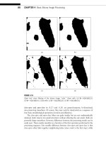
Figure 21.13 illustrates spatial quality maps generated by VIF. Figure 21.13(a) shows
a reference image and Fig. 21.13(b) the corresponding JPEG2000 compressed image
in which the distortions are clearly visible. Figure 21.13(c) shows the reference image
information map. The information map shows the spread of statistical information in
the reference image. The statistical information content of the image is low in flat image
regions, whereas in textured regions and regions containing strong edges, it is high. The
quality map in Fig. 21.13(d) shows the proportion of the image information that has
been lost to JPEG2000 compression. Note that due to the nonlinear normalization in the
denominator of VIF, the scalar VIF value for a reference/test pair is not the mean of the
corresponding VIF-map.

21.4.3 Relation to HVS-Based Metrics and Structural Similarity
We will first discuss therelation between IFCand SSIM index [13, 17]. First of all, the GSM
model used in the information theoretic metrics results in the subband coefficients being
Gaussian distributed, when conditioned on a fixed mixing multiplier in the GSM model.
The linear distortion channel model results in the reference and test images being jointly
Gaussian. The definition of the correlation coefficient in the SSIM index in (21.19) is
obtained from regression analysis and implicitly assumes that the reference and test image
vectors are jointly Gaussian [22].Infact,(21.19) coincides with the maximum likelihood
estimate of the correlation coefficient only under the assumption that the reference and
distorted image patches are jointly Gaussian distributed [22]. These observations hint at
the possibility that the IFC index may be closely related to SSIM. A well-known result
in information theory states that when two variables are jointly Gaussian, the mutual
information between them is a function of just the correlation coefficient [23, 24]. Thus,
recent results show that a scalar version of the IFC metric is a monotonic function of
the square of the structure term of the SSIM index when the SSIM index is applied
on subband filtered coefficients [13, 17]. The reasons for the monotonic relationship
between the SSIM index and the IFC index are the explicit assumption of a Gaussian
distribution on the reference and test image coefficients in the IFC index (conditioned
on a fixed mixing multiplier) and the implicit assumption of a Gaussian distribution in
the SSIM index (due to the use of regression analysis). These results indicate that the IFC
index is equivalent to multiscale SSIM indices since they satisfy a monotonic relationship.
Further, the concept of the correlation coefficient in SSIM was generalized to vector
valued variables using canonical correlation analysis to establish a monotonic relation
between the squares of the canonical correlation coefficients and the vector IFC index
586 CHAPTER 21 Image Quality Assessment
(a) Reference image (b) JPEG2000 compressed
(c) Reference image info. map (d) VIF map
FIGURE 21.13
Spatial maps showing how VIF captures spatial information loss.
[13, 17]. It was also established that the VIF index includes a structure comparison term

and a contrast comparison term (similar to the SSIM index), as opposed to just the
structure term in IFC. One of the properties of the VIF index observed in Section 21.4.2
was the fact that it can predict improvement in quality due to contrast enhancement. The
presence of the contrast comparison term in VIF explains this effect [13, 17].
We showed the relation between SSIM- and HVS-based metrics in Section 21.3.3.
From our discussion here, the relation between IFC-, VIF-, and HVS-based metrics is
21.5 Performance of Image Quality Metrics 587
also immediately apparent. Similarities between the scalar IFC index and the HVS-based
metrics were also observed in [26]. It was shown that the IFC is functionally similar to
HVS-based FR QA algorithms [26]. The reader is referred to [13, 17] for a more thorough
treatment of this subject.
Having discussed the similarities between the SSIM and the information theoretic
frameworks, we will now discuss the differences between them. The SSIM metrics use
a measure of linear dependence between the reference and test image pixels, namely
the Pearson product moment correlation coefficient. However, the information theoretic
metrics use the mutual information, which is a more general measure of correlation that
can capture nonlinear dependencies between variables. The reason for the monotonic
relation between the square of the structure term of the SSIM index applied in the
subband filtered domain and the IFC index is due to the assumption that the reference
and test image coefficients are jointly Gaussian. This indicates that the structure term of
SSIM and IFC is equivalent under the statistical source model used in [26], and more
sophisticated statistical models are required in the IFC framework to distinguish it from
the SSIM index.
Although the information theoretic metrics use a more general and flexible notion of
correlation than the SSIM philosophy, the form of the relationship between the reference
and test images might affect visual quality. As an example, if one test image is a determin-
istic linear function of the reference image, while another test image is a deterministic
parabolic function of the reference image, the mutual information between the reference
and the test image is identical in both cases. However, it is unlikely that the visual quality
of both images is identical. We believe that further investigation of suitable models for

the distortion channel and the relation between such channel models and visual quality
are required to answer this question.
21.5 PERFORMANCE OF IMAGE QUALITY METRICS
In this section, we present results on the validation of some of the image quality metrics
presented in this chapter and present comparisons with PSNR. All results use the LIVE
image QA database [8] developed by Bovik and coworkers and further details can be
found in [7]. The validation is done using subjective quality scores obtained from a
group of human observers, and the performance of the QA algorithms is evaluated by
comparing the quality predictions of the algorithms against subjective scores.
In the LIVE database, 20–28 human subjects were asked to assign each image
with a score indicating their assessment of the quality of that image, defined as the
extent to which the artifacts were visible and annoying. Twenty-nine high-resolution
24-bits/pixel RGB color images (ty pically 768 ϫ 512) were distorted using five distortion
types: JPEG2000, JPEG, white noise in the RGB components, Gaussian blur, and trans-
mission errors in the JPEG2000 bit stream using a fast-fading Rayleigh channel model.
A database was derived from the 29 images to yield a total of 779 distorted images, which,
together with the undistorted images, were then evaluated by human subjects. The raw
scores were processed to y ield difference mean opinion scores for validation and testing.
588 CHAPTER 21 Image Quality Assessment
TABLE 21.1 Performance of different QA methods
Performance
Model LCC SROCC
PSNR 0.8709 0.8755
Sarnoff JND 0.9266 0.9291
Multiscale SSIM 0.9393 0.9527
IFC 0.9441 0.9459
VIF 0.9533 0.9584
VSNR 0.9233 0.9278
Usually, the predicted quality scores from a QA method are fitted to the subjective
quality scores using a monotonic nonlinear function to account for any nonlinearities

in the objective model. Numerical methods are used to do this fitting. For the results
presented here, a five-parameter nonlinearity (a logistic function with additive linear
term) was used, and the mapping function used is given by
Quality(x) ϭ ␤
1
logistic
(
␤
2
,(x Ϫ ␤
3
)
)
ϩ ␤
4
x ϩ ␤
5
, (21.45)
logistic(␶, x) ϭ
1
2
Ϫ
1
1 ϩ ex p(␶x)
. (21.46)
Table 21.1 quantifies the performance of the various methods in terms of well-known
validation quantities: the linear correlation coefficient (LCC) between objective model
prediction and subjective quality and the Spearman rank order correlation coefficient
(SROCC) between them. Clearly, several of these quality metrics correlate very well with
visual perception. The performance of IFC and multiscale SSIM indices is comparable,

which is not surprising in view of the discussion in Section 21.4.3. Interestingly, the
SSIM index correlates very well with visual perception despite its simplicity and ease of
computation.
21.6 CONCLUSION
Hopefully, the reader has captured an understanding of the basic principles and difficul-
ties underlying the problem of image QA. Even when there is a reference image available,
as we have assumed in this chapter, the problem remains difficult owing to the subtleties
and remaining mysteries of human visual perception. Hopefully, the reader has also
found that recent progress has been significant, and that image QA algorithms exist that
correlate quite highly with human judgments. Ultimately, it is hoped that confidence in
these algorithms will become high enough that image quality algorithms can be used as
surrogates for human subjectivity.
References 589
Naturally, significant problems remain. The use of partial image information instead
of areferenceimage—so-called reducedreferenceimage QA—presents interestingoppor-
tunities where good performance can be achieved in realistic applications where only
partial data about the reference image may be available. More difficult yet is the situation
where no reference image information is available. This problem, called no-reference or
blind image QA, is very difficult to approach unless there is at least some information
regarding the types of distortions that might be encountered [5].
An interesting direction for future work is the further use of image QA algorithms as
objective functions for image optimization problems. For example, the SSIM index has
been used to optimize several important image processing problems, including image
restoration, image quantization, and image denoising [9–12]. Another interesting line
of inquiry is the use of image quality algorithms—or variations of them—for other
purposes than image quality assessment—such as speech quality assessment [4].
Lastly, we have not covered methods for assessing the quality of digital videos. There
are many sources of distortion that may occur owing to time-dependent processing of
videos, and interesting aspects of spatio-temporal visual perception come into play when
developing algorithms for video QA. Such algorithms are by necessity more involved

in their construction and complex in their execution. The reader is encouraged to read
Chapter 14 of the companion volume, The Essential Guide to Video Processing, for a
thorough discussion of this topic.
REFERENCES
[1] Z. Wang and X. Shang. Spatial pooling strategies for perceptual image quality assessment. In IEEE
International Conference on Image Processing. IEEE, Dept. of EE, Texas Univ. at Arlington, TX,
USA, January 1996.
[2] Z. Wang and A. C. Bovik. Embedded foveation image coding. IEEE Trans. Image Process.,
10(10):1397–1410, 2001.
[3] Z. Wang, L. Lu, and A. C. Bovik. Foveation scalable video coding with automatic fixation selection.
IEEE Trans. Image Process., 12(2):243–254, 2003.
[4] Z. Wang and A. C. Bovik. Mean squared error: love it or leave it? A new look at signal fidelity
measures. IEEE Signal Process. Mag., to appear, January 2009.
[5] Z. Wang and A. C. Bovik. Modern Image Quality Assessment. Morgan and Claypool Publishing
Co., San Rafael, CA, 2006.
[6] A. B. Watson. DCTune: a technique for visual optimization of dct quantization matrices for
individual images. Soc. Inf. Disp. Dig. Tech. Pap., 24:946–949, 1993.
[7] H. R. Sheikh, M. F. Sabir, and A. Bovik. A statistical evaluation of recent full reference image
quality assessment algorithms. IEEE Trans. Image Process., 15(11):3440–3451, 2006.
[8] LIVE image quality assessment database. 2003. />subjective.htm
[9] S. S. Channappayya,A. C.Bovik,andR. W. Heath,Jr.A linear estimatoroptimized forthestructural
similarity index and its application to image denoising. In IEEE Intl. Conf. Image Process., Atlanta,
GA, January 2006.
590 CHAPTER 21 Image Quality Assessment
[10] S. S. Channappayya, A. C. Bovik, C. Caramanis, and R. W. Heath, Jr. Design of linear equalizers
optimized for the structural similarit y index. IEEE Trans. Image Process., to appear, 2008.
[11] S. S. Channappayya, A. C. Bovik, and R. W. Heath, Jr. Rate bounds on SSIM index of quantized
images. IEEE Trans. Image Process., to appear, 2008.
[12] S. S. Channappayya, A. C. Bovik, R. W. Heath, Jr., and C. Caramanis. Rate bounds on the SSIM
index of quantized image DCT coefficients. In Data Compression Conf., Snowbird, Utah, March

2008.
[13] K. Seshadrinathan and A. C. Bovik. Unifying analysis of full reference image quality assessment.
To appear in IEEE Intl. Conf. on Image Process., 2008.
[14] M. J. Wainwright, E. P. Simoncelli, and A. S. Willsky. Random cascades on wavelet trees and their
use in analyzing and modeling natural images. Appl. Comput. Harmonic Anal., 11(1):89–123,
2001.
[15] E. P. Simoncelli and W. T. Freeman. The steerable pyramid: a flexible architecture for multi-scale
derivative computation. In Proc. Intl. Conf. on Image Process., Vol. 3, January 1995.
[16] Z. Wang and E. P. Simoncelli. Stimulus synthesis for efficient evaluation and refinement of
perceptual image quality metrics. Proc. SPIE, 5292(1):99–108, 2004.
[17] K. Seshadrinathan and A. C. Bovik. Unified treatment of full reference image quality assessment
algorithms. Submitted to the IEEE Trans. on Image Process.
[18] D. J. Heeger. Normalization of cell responses in cat striate cortex. Vis. Neurosci., 9(2):181–197,
1992.
[19] Z. Wang, E. P. Simoncelli, and A. C. Bovik. Multiscale structural similarity for image quality
assessment. In Thirty-Seventh Asilomar Conf. on Signals, Systems and Computers, Pacific Grove,
CA, 2003.
[20] Z. Wang and E. P. Simoncelli. Translation insensitive image similarity in complex wavelet domain.
In IEEE Intl. Conf. Acoustics, Speech, and Signal Process., Philadelphia, PA, 2005.
[21] M. J. Wainwright and E. P. Simoncelli. Scale mixtures of gaussians and the statistics of natural
images. In S. A. Solla, T. Leen, and S R. Muller, editors, Advance Neural Information Processing
Systems, 12:855–861, MIT Press, Cambridge, MA, 1999.
[22] T. W. Anderson.An Introduction to Multivariate Statistical Analysis. JohnWiley andSons,NewYork,
1984.
[23] I. M. Gelfand and A. M. Yaglom. Calculation of the amount of information about a random
function contained in another such function. Amer. Math. Soc. Transl., 12(2):199–246, 1959.
[24] S. Kullback. Information Theory and Statist ics. Dover Publications, Mineola, NY, 1968.
[25] H. R. Sheikh and A. C. Bovik. Image information and visual quality. IEEE Trans. Image Process.,
15(2):430–444, 2006.
[26] H. R. Sheikh, A. C. Bovik, and G. de Veciana. An information fidelity criterion for image quality

assessment using natural scene statistics. IEEE Trans. Image Process., 14(12):2117–2128, 2005.
[27] J. Ross and H. D. Speed. Contrast adaptation and contrast masking in human vision. Proc. Biol.
Sci., 246(1315):61–70, 1991.
[28] Z. Wang and A. C. Bovik. A universal image quality index. IEEE Signal Process. Lett., 9(3):81–84,
2002.
[29] Z. Wang, A. C. Bovik, H. R. Sheikh, and E. P. Simoncelli. Image quality assessment: from error
visibility to structural similarity. IEEE Trans. Image Process., 13(4):600–612, 2004.
References 591
[30] D. M. Chandler and S. S. Hemami. VSNR: a wavelet-based visual signal-to-noise ratio for natur al
images. IEEE Trans. Image Process., 16(9):2284–2298, 2007.
[31] A. Watson and J. Solomon. Model of v isual contrast gain control and pattern masking. J. Opt. Soc.
Am. A Opt. Image Sci. Vis., 14(9):2379–2391, 1997.
[32] O. Schwartz and E. P. Simoncelli. Natural signal statistics and sensory gain control. Nat. Neurosci.,
4(8):819–825, 2001.
[33] J. Foley. Human luminance pattern-vision mechanisms: masking experiments require a new
model. J. Opt. Soc. Am. A Opt. Image Sci. Vis., 11(6):1710–1719, 1994.
[34] D. G. Albrecht and W. S. Geisler. Motion selectivity and the contrast-response function of simple
cells in the visual cortex. Vis. Neurosci., 7(6):531–546, 1991.
[35] R. Shapley and C. Enroth-Cugell. Visual adaptation and retinal gain controls. Prog. Retin. Res.,
3:263–346, 1984.
[36] T. N. Pappas, T. A. Michel, and R. O. Hinds. Supra-threshold perceptual image coding. In Proc.
Int. Conf. Image Processing (ICIP-96), Vol. I, 237–240, Lausanne, Switzerland, September 1996.
[37] S. Daly. The visible differences predictor: an algorithm for the assessment of image fidelity.
In A. B. Watson, editor, Digital Images and Human Vision, 179–206. The MIT Press, Cambridge,
MA, 1993.
[38] J. Lubin. The use of psychophysical data and models in the analysis of display system performance.
In A. B. Watson, editor, Digital Images and Human Vision, 163–178. The MIT Press, Cambridge,
MA, 1993.
[39] P. C. Teo and D. J. Heeger. Perceptual image distortion. In Proc. Int. Conf. Image Processing
(ICIP-94), Vol. II, 982–986, Austin, TX, November 1994.

[40] R. J. Safranek and J. D. Johnston. A perceptually tuned sub-band image coder with image depen-
dent quantization and post-quantization data compression. In Proc. ICASSP-89, Vol. 3, Glasgow,
Scotland, 1945–1948, May 1989.
[41] A. B. Watson. DCT quantization matr ices visually optimized for individual images. In J. P.Allebach
and B. E. Rogowitz, editors, Human Vision, Visual Processing, and Digital Display IV, Proc. SPIE,
1913, 202–216, San Jose, CA, 1993.
[42] R. J. Safranek. A JPEG compliant encoder utilizing perceptually based quantization. In
B. E. Rogowitz and J. P. Allebach, editors, Human Vision, Visual Processing, and Digital Display V,
Proc. SPIE, 2179, 117–126, San Jose, CA, 1994.
[43] D. L. Neuhoff and T. N. Pappas. Perceptual coding of images for halftone display. IEEE Trans.
Image Process., 3:341–354, 1994.
[44] R. Rosenholtz and A. B. Watson. Perceptual adaptive JPEG coding. In Proc. Int. Conf. Image
Processing (ICIP-96) , Vol. I, 901–904, Lausanne, Switzerland, September 1996.
[45] I. Höntsch and L. J. Karam. Apic: adaptive perceptual image coding based on subband decompo-
sition with locally adaptive perceptual weighting. In Proc. Int. Conf. Image Processing (ICIP-97),
Vol. I, 37–40, Santa Barbara, CA, October 1997.
[46] I. Höntsch, L. J. Karam, and R. J. Safranek. A p erceptually tuned embedded zerotree image coder.
In Proc. Int. Conf. Image Processing (ICIP-97), Vol. I, 41–44, Santa Barbara, CA, October 1997.
[47] I. Höntsch and L. J. Karam. Locally adaptive perceptual image coding. IEEE Trans. Image Process.,
9:1472–1483, 2000.
[48] I. Höntsch and L. J. Karam. Adaptive image coding with perceptual distortion control. IEEE Trans.
Image Process., 9:1472–1483, 2000.
592 CHAPTER 21 Image Quality Assessment
[49] A. B. Watson, G. Y. Yang, J. A. Solomon, and J. Villasenor. Visibility of wavelet quantization noise.
IEEE Trans. Image Process., 6:1164–1175, 1997.
[50] P. G. J. Barten. The SQRI method: a new method for the evaluation of visible resolution on a
display. In Proc. Society for Information Display, Vol. 28, 253–262, 1987.
[51] J. Sullivan, L. Ray, and R. Miller. Design of minimum visual modulation halftone patterns. IEEE
Trans. Syst., Man, Cybern., 21:33–38, 1991.
[52] M. Analoui and J. P.Allebach. Model based halftoning usingdirect binary search. In B. E.Rogowitz,

editor,Human Vision,Visual Processing, and Digital Display III, Proc. SPIE, 1666, 96–108, San Jose,
CA, 1992.
[53] J. B. Mulligan and A. J. Ahumada, Jr. Principled halftoning based on models of human vision. In
B. E. Rogowitz, editor, Human Vision, Visual Processing, and Digital Display III, Proc. SPIE, 1666,
109–121, San Jose, CA, 1992.
[54] T. N. Pappas and D. L. Neuhoff. Least-squares model-based halftoning. In B. E. Rogowitz, editor,
Human Vision, Visual Processing, and Digital Display III, Proc. SPIE, 1666, 165–176, San Jose, CA,
1992.
[55] T. N. Pappas and D. L. Neuhoff. Least-squares model-based halftoning. IEEE Trans. Image Process.,
8:1102–1116, 1999.
[56] R. Hamberg and H. de Ridder. Continuous assessment of time-varying image quality. In
B. E. Rogowitz and T. N. Pappas, editors, Human Vision and Electronic Imaging II, Proc. SPIE,
3016, 248–259, San Jose, CA, 1997.
[57] H. de Ridder. Psychophysical evaluation of image quality: from judgement to impression. In
B. E. Rogowitz and T. N. Pappas, editors, Human Vision and Electronic Imaging III, Proc. SPIE,
3299, 252–263, San Jose, CA, 1998.
[58] ITU/R Recommendation BT.500-7, 10/1995. .
[59] T. N. Cornsweet. Visual Perception. Academic Press, New York, 1970.
[60] C. F. Hall and E. L. Hall. A nonlinear model for the spatial characteristics of the human visual
system. IEEE Trans. Syst., Man. Cybern., SMC-7:162–170, 1977.
[61] T. J. Stockham. Image processing in the context of a v isual model. Proc. IEEE, 60:828–842, 1972.
[62] J. L. Mannos and D. J. Sakrison. The effects of a visual fidelit y criterion on the encoding of images.
IEEE Trans. Inform. Theory, IT-20:525–536, 1974.
[63] J. J. McCann, S. P. McKee, and T. H. Taylor. Quantitative studies in the retinex theory. Vision Res.,
16:445–458, 1976.
[64] J. G. Robson and N. Graham. Probability summation and regional variation in contrast sensitivity
across the visual field. Vision Res., 21:419–418, 1981.
[65] G. E. Legge and J. M. Foley. Contrast masking in human vision. J Opt Soc Am, 70(12):1458–1471,
1980.
[66] G. E. Legge. A power law for contrast discrimination. Vision Res., 21:457–467, 1981.

[67] B. G. Breitmeyer. Visual Masking: An Integrative Approach. Oxford University Press, New York,
1984.
[68] A. J. Seyler and Z. L. Budrikas. Detail perception after scene change in television image
presentations. IEEE Trans. Inform. Theory, IT-11(1):31–43, 1965.
[69] Y. Ninomiya,T. Fujio,and F. Namimoto. Perceptionof impairment by bit reduction oncut-changes
in television pictures. (in Japanese). Electr. Commun. Assoc. Essay Periodical, J62-B(6):527–534,
1979.
References 593
[70] W. J. Tam, L. Stelmach, L. Wang, D. Lauzon, and P. Gray. Visual masking at video scene cuts. In
B. E. Rogowitz and J. P. Allebach, editors, Proceedings of the SPIE Conference on Human Vision,
Visual Processing and Digital Display VI, Proc. SPIE, 2411, 111–119, San Jose, CA, 1995.
[71] D. H. Kelly. Visual response to time-dependent stimuli. J. Opt. Soc. Am., 51:422–429, 1961.
[72] D. H. Kelly. Flicker fusion and harmonic analysis. J. Opt. Soc. Am., 51:917–918, 1961.
[73] D. H. Kelly. Flickering patterns and lateral inhibition. J. Opt. Soc. Am., 59:1361–1370, 1961.
[74] D. A. Silverstein and J. E. Farrell. The relationship between image fidelity and image quality. In
Proc. Int. Conf. Image Processing (ICIP-96), Vol. II, 881–884, Lausanne, Switzerland, September
1996.
[75] C. A. Poynton. A Technical Introduction to Digital Video. Wiley, New Yor k, 1996.
[76] A. B. Watson. The cortex transform: rapid computation of simulated neural images. Comput.
Vision, Graphics, and Image Process., 39:311–327, 1987.
[77] P. J. Burt and E. H. Adelson. The Laplacian pyramid as a compact image code. IEEE Trans.
Commun., 31:532–540, 1983.
[78] W. T. Freeman and E. H. Adelson. The design and use of steerable filters. IEEE Trans. Pattern Anal.
Mach. Intell., 13:891–906, 1991.
[79] E. P. Simoncelli, W. T. Freeman, E. H. Adelson, and D. J. Heeger. Shiftable multiscale transforms.
IEEE Trans. Inform. Theory, 38:587–607, 1992.
[80] P. C. Teo and D. J. Heeger. Perceptual image distortion. In B. E . Rogowitz and J. P. Allebach,editors,
Human Vision, Visual Processing, and Digital Display V, Proc. SPIE, 2179, 127–141, San Jose, CA,
1994.
[81] R. J. Safr anek. A comparison of the coding efficiency of perceptual models. In Human Vision,

Visual Processing, and Digital Display VI, Proc. SPIE, 2411, 83–91, San Jose, CA, February 1995.
[82] C. J. van den Branden Lambrecht and O. Verscheure. Perceptual quality measure using a spatio-
temporal model of the human visual system. InV. Bhaskaran, F. Sijstermans, and S. Panchanathan,
editors, Digital Video Compression: Algorithms and Technologies, Proc. SPIE, 2668, 450–461,
San Jose, CA, January/February 1996.
[83] J. Chen and T. N. Pappas. Perceptual coders and perceptual metrics. In B. E. Rogowitz and
T. N. Pappas, editors, Human Vision and Electronic Imaging VI, Proc. SPIE, 4299, 150–162, San
Jose, CA, January 2001.
[84] A. Said and W. A. Pearlman. A new fast and efficient image codec based on set partitioning in
hierarchical trees. IEEE Trans. Circuits Syst. Video Technol., 6:243–250, 1996.
[85] H. A. Peterson, A. J. Ahumada, Jr., and A. B. Watson. An improved detection model for DCT
coefficient quantization. In J. P. Allebach and B. E. Rogowitz, editors, Human Vision, Visual
Processing, and Digital Display IV, Proc. SPIE, 1913, 191–201, San Jose, CA, 1993.
[86] B. E. Usevitch. A tutorial on modern lossy wavelet image compression: foundations of JPEG 2000.
IEEE Signal Process. Mag., 18:22–35, 2001.
[87] A. Skodras, C. Christopoulos, and T. Ebrahimi. The JPEG 2000 still image compression standard.
IEEE Signal Process. Mag., 18:36–58, 2001.
[88] D. S. Taubman and M. W. Marcellin. JPEG2000: standard for interactive imaging. Proc. IEEE,
90:1336–1357, 2002.
[89] J. M. Shapiro. Embedded image coding using zerotrees of wavelet coefficients. IEEE Trans. Signal
Process., SP-41:3445–3462, 1993.
594 CHAPTER 21 Image Quality Assessment
[90] D. Taubman. High performance scalable image compression with ebcot. IEEE Trans. Image
Process., 9:1158–1170, 2000.
[91] A. Cohen, I. Daubechies, and J. C. Feauveau. Biorthogonal bases of compactly supported wavelets.
Commun. Pure Appl. Math., 45:485–560, 1992.
[92] A. J. Ahumada, Jr. and H. A. Peterson. A visual detection model for DCT coefficient quantization.
In AIAA Computing in Aerospace 9: A Collection of Technical Papers, 314–317, San Diego, CA,
October 1993.
[93] M. P. Eckert and A. P. Bradley. Perceptual quality metrics applied to still image compression.

Signal Process., 70:177–200, 1998.
[94] S. Daly. Subroutine for the generation of a two dimensional human visual contrast sensitivity
function. Technical Report 233203Y, Eastman Kodak, Rochester, NY, 1987.
[95] D. A. Silverstein and S. A. Klein. A DCT image fidelity metric for application to a text-based
scheme for image display. In J. P. Allebach and B. E. Rogowitz, editors, Human Vision, Visual
Processing, and Digital Display IV, Proc. SPIE, 1913, 229–239, San Jose, CA, 1993.
[96] S. J. P. Westen, R. L. Lagendijk, and J. Biemond. Perceptual image quality based on a multiple
channel HVS model. In Proc. ICASSP-95, Vol. 4, 2351–2354, Detroit, MI, May 1995.
[97] M. J. Horowitz and D. L. Neuhoff. Image coding by perceptual pruning with a cortical snapshot
indistinguishability criterion. In B. E. Rogowitz and T. N. Pappas, editors, Human Vision and
Electronic Imaging III, Proc. SPIE, 3299, 330–339, San Jose, CA, 1998.
[98] N. Bekkat and A. Saadane. Coded image quality assessment based on a new contrast masking
model. J. Electron. Imaging, 13:341–348, 2004.
[99] S. Winkler and S. Süsstrunk. Visibility of noise in natural images. In Human Vision and Electronic
Imaging IX, Proc. SPIE, 5292, San Jose, CA, January 2004.
[100] C. Fenimore, B. Field, and C. V. Degrift. Test patterns and quality metrics for digital video com-
pression. In B. E. Rogowitz and T. N. Pappas, editors, Human Vision and Electronic Imaging II,
Proc. SPIE, 3016, 269–276, San Jose, CA, February 1997.
[101] J. M. Libert and C. Fenimore. Visibility thresholds for compression-induced image blocking:
measurement andmodels.In B.E.Rogowitz and T. N. Pappas,editors,HumanVisionandElectronic
Imaging IV, Proc. SPIE, 3644, 197–206, San Jose, CA, January 1999.
[102] E. M. Yeh, A. C. Kokaram, and N. G. Kingsbury. A perceptual distortion measure for edge-like
artifacts in image sequences. In B. E. Rogowitz and T. N. Pappas, editors, Human Vision and
Electronic Imaging III, Proc. SPIE, 3299, 160–172, San Jose, CA, January 1998.
[103] P. J. Hahn and V. J. Mathews. An analytical model of the perceptual threshold function for
multichannel image compression. In Proc. Int. Conf. Image Processing (ICIP-98), Vol. III, 404–408,
Chicago, IL, October 1998.
[104] M. G. Ramos and S. S. Hemami. Suprathreshold wavelet coefficient quantization in complex
stimuli: psychophysical evaluation and analysis. J. Opt. Soc. Am. A, 18:2385–2397, 2001.
[105] D. M. Chandler and S. S. Hemami. Additivity models for suprathreshold distortion in quantized

wavelet-coded images. In B. E. Rogowitz and T. N. Pappas, editors, Human Vision and Electronic
Imaging VII, Proc. SPIE, 4662, 105–118, San Jose, CA, January 2002.
[106] D. M. Chandler and S. S. Hemami. Effects of natural images on the detectability of simple and
compound wavelet subband quantization distortions. J. Opt. Soc. Am. A, 20(7):1164–1180, 2003.
[107] D. M. Chandler and S. S. Hemami. Suprathreshold image compression based on contrast allo-
cation and global precedence. In B. E. Rogowitz and T. N. Pappas, editors, Human Vision and
Electronic Imaging VIII, Proc. SPIE, 5007, Santa Clara, CA, January 2003.
References 595
[108] D. M.Chandlerand S. S. Hemami. Contrast-based quantization and ratecontrolforwavelet-coded
images. In Proc. Int. Conf. Image Processing (ICIP-02), Rochester, NY, September 2002.
[109] T. N. Pappas, J. P. Allebach, and D. L. Neuhoff. Model-based digital halftoning. IEEE Signal Process.
Mag., 20:14–27, 2003.
[110] W. Qian and B. Kimia. On the perceptual notion of scale for halftone representations: nonlinear
diffusion. In B. E. Rogowitz and T. N. Pappas, editors, Human Vision and Electronic Imaging, Proc.
SPIE, 3299, 473–481, San Jose, CA, January 1998.
[111] P. Lindh and C. J. van den Branden Lambrecht. Efficient spatio-temporal decomposition for
perceptual processing of video sequences. In Proc. Int. Conf. Image Processing (ICIP-96), Vol. III,
331–334, Lausanne, Switzerland, September 1996.
[112] S. Winkler. Quality metric design: a closer look. In B. E. Rogowitz and T. N. Pappas, editors,
Human Vision and Electronic Imaging V, Proc. SPIE, 3959, San Jose, CA, January 2000.
[113] S. Winkler.Visual fidelity and perceived quality: towards comprehensive metrics. In B. E. Rogowitz
and T. N. Pappas, editors, Human Vision and Electronic Imaging VI, Proc. SPIE, 4299, San Jose,
CA, January 2001.
[114] A. M. Rohaly, J. Lu, N. R. Franzen, and M. K. Ravel. Comparison of temporal pooling methods for
estimating the quality of complex video sequences. In B. E. Rogowitz and T. N. Pappas, editors,
Human Vision and Electronic Imaging IV, Proc. SPIE, 3644, 218–225, San Jose, CA, January 1999.
[115] D. Pearson. Viewer response to time-varying video quality. In B. E. Rogowitz and T. N. Pappas,
editors, Human Vision and Electronic Imaging III, Proc. SPIE, 3299, 16–25, San Jose, CA, January
1998.
[116] A. B. Watson. Toward aperceptual video quality metric. In B.E.Rogowitz and T. N. Pappas,editors,

Human Vision and Electronic Imaging III, Proc. SPIE, 3299, 139–147, San Jose, CA, Januar y 1998.
[117] A. B. Watson, J. Hu, and J. F. McGowan, III. Digital video quality metric based on human vision.
J. Electron. Imaging, 10:20–29, 2001.
[118] A. B. Watson, J. Hu, J. F. McGowan, and J. B. Mulligan. Design and performance of a digital video
quality metric. In B. E. Rogowitz and T. N. Pappas, editors, Human Vision and Electronic Imaging
IV, Proc. SPIE, 3644, 168–174, San Jose, CA, January 1999.
[119] R. O. Hinds and T. N. Pappas. Effect of concealment techniques on perceived video qualit y. In
B. E. Rogowitz and T. N. Pappas, editors, Human Vision and Electronic Imaging IV, Proc. SPIE,
3644, 207–217, San Jose, CA, January 1999.
[120] K. Brunnström and B. N. Schenkman. Quality of video affected by packet loss distortion, com-
pared to the predictions of a spatio-temporal model. In B. E. Rogowitz and T. N. Pappas, editors,
Human Vision and Electronic Imaging VII, Proc. SPIE, 4662, San Jose, CA, January 2002.
CHAPTER
22
Image Watermarking:
Techniques and
Applications
Anastasios Tefas, Nikos Nikolaidis, and Ioannis Pitas
Aristotle University of Thessaloniki
22.1 INTRODUCTION
Digital watermarking is a relatively new research area that has attracted the interest
of numerous researchers both in academia and industry and has become one of the
hottest research topics in the multimedia signal processing community. Although the
term watermarking has slightly different meanings in the literature, one definition that
seems to prevail is the following [1]: Watermarking is the practice of imperceptibly alter-
ing a piece of data in order to embed information about the data. The above definition
reveals two important characteristics of watermarking. First, information embedding
should not cause perceptible changes to the host medium (sometimes called cover
medium or cover data). Second, the message should be related to the host medium.
In this sense, the watermarking techniques form a subset of information hiding tech-

niques, which also include cases where the hidden information is not related to the
host medium (e.g., in covert communications). However, certain authors use the term
watermarking with a meaning equivalent to that of information hiding in the general
sense.
A watermarking system should consist of two distinct modules: a module that embeds
the information in the host data and a module that detects if a given piece of data hosts a
watermark and subsequently retrieves the conveyed information. Depending on the type,
the amount, and the properties of the embedded information (e.g., robustness to host
signal alterations), as well as the type of host data, watermarking can serve a multitude
of applications as will be described in Section 22.2.
The first handful of papers on dig ital watermarking appeared in the late 1980s-early
1990s but ver y soon the area witnessed a tremendous growth and an explosion in the
number of published papers, mainly due to the fact that people believed, at that stage, that
watermarking could be a significant weapon in the battle against continuously increas-
ing digital media piracy. During the early days, researchers focused mainly on a limited
597
598 CHAPTER 22 Image Watermarking: Techniques and Applications
range of host data, that is, digital image, video, and audio data. Later on, watermar king
techniques that are applicable to other media types appeared in the corresponding
literature. Such media types include but are not limited to voxel-based 3D images, 3D
models represented as polygonal meshes or parametric surfaces (e.g., NURBS surfaces),
vector graphics, GIS data (e.g., isosurface contours), animation parameters, object-based
video representations (e.g., MPEG 4 video objects), symbolic description of audio (e.g.,
MIDI files), text (either in ASCII format or as a binary image), software source code,
binary executables, java byte code, and numeric data sets (stock market data, scientific
data). This chapterwill focus on still image watermarking. However,most of the principles
and techniques that will be presented are readily applicable to other media types.
Although, in its first steps, watermarking was dominated by heuristic approaches
without significant theoretical background and justification, soon researchers recog-
nized that solid theoretical foundations had to be set and worked toward this direction

by adopting and utilizing successful techniques, principles, and theoretical results from
several scientific areas like communications (detection theory, error correction codes,
spread spectrum communications), infor mation theory (channel capacity), signal pro-
cessing (signal transforms, compression techniques), and cryptography. Today, although
the optimism of the early years is over, watermarking is still a very active research area,
despite the failure of the cur rently available watermarking technology to serve the needs
of the industry (as made clear by Secure Digital Music Initiative case [2]). Researchers
are now very well aware that devising effective watermarking schemes, especially for the
so-called security oriented applications (e.g., copyright protection, copy control, etc.), is
an extremely difficult task. However, the introduction of new application scenarios and
business models along with the small but steady steps toward solid theoretical founda-
tions of this discipline and the combination of watermarking with other technologies
like cryptography and perceptual hashing [3–5] are expected to keep the interest in this
new area alive [6, 7]. For a thorough review of existing schemes and a detailed discussion
on the main requirements of a watermarking scheme, the interested reader may con-
sult books [1, 8–11] and several review papers and journal special issues [12–17] that
have been published on this topic. The IEEE Transactions on Information Forensics and
Security is another excellent source of information regarding the latest developments in
the field.
This chapter is organized as follows. The main application domains of watermarking
are reviewed in Section 22.2. Properties and classification schemes of watermarking tech-
niques are presented in Section 22.3, whereas Section 22.4 presents the basic functional
modules of a watermarking scheme. Finally Sections 22.5 and 22.6 delve in more detail
into principles and techniques devised for two major application areas, namely copyright
protection and authentication.
22.2 APPLICATIONS OF WATERMARKING TECHNIQUES
Watermarking can be the enabling technology for a number of important appli-
cations [18–20]. Obviously, each application imposes different requirements on the
22.2 Applications of Watermarking Techniques 599
watermarking system. As a consequence, watermarking algorithms targeting different

applications might be very different in nature. Furthermore, devising an efficient
watermarking scheme might be much more difficult for certain applications. In the
remainder of this section, we will briefly review some of the main application domains
of watermarking.
■ Owner identification and proof of ownership. This class of applications was the first
to be considered in the watermarking literature. In this case, the embedded data
can carry information about the legal owner or distributor or any rights holder of
a digital item and be used for notifying/warning a user that the item is copyrighted,
for tracking illegal copies of the item, or for possibly proving the ownership of the
item in the case of a legal dispute.
■ Broadcast monitoring. In this case, the embedded information is utilized for various
functions that are related to digital media (audio, video) broadcasting. The embed-
ded data can be used to verify whether the actual broadcasting of commercials took
place as scheduled, i.e., whether proper airtime allocation occurred, for devising
an automated royalty collection scheme for copyrighted material (songs, movies)
that is aired by broadcasting operators, or to collect information about the num-
ber of people who watched/listened to a certain broadcast (audience metering).
Broadcast monitoring is usually performed by automated monitoring stations and
is one of the watermarking applications that has found its way toward successful
commercialization.
■ Transaction tracking. In this application, each copy of a digital item that is dis-
tributed as part of a transaction bears a different watermark. The aim of this
watermark is not only to carry information about the legal owner/distributor
of the digital item but also to mark the specific transaction copy. As a conseq-
uence, the embedded information can be used for the identification of entities that
illegally distributed the digital item or did not adopt efficient security measures
for preventing the item from being copied or distributed and for deterring such
actions. Identification of movie theaters where illegal recording of a movie with
a handheld camera took place is a scenario that belongs to this category of appli-
cations. The watermarks used in such cases are often termed fingerprints and the

corresponding application fingerprinting. However, the same term is sometimes
used for the class of techniques that try to extract a unique descriptor (fingerprint)
for each digital item, which is invariant to content manipulation [3–5, 21].Obvi-
ously these techniques (which are sometimes called perceptual or robust hashing
or replica detection techniques) are totally different from watermark-based finger-
printing, since they do not embed any data on the digital item, i.e., they are passive
techniques.
■ Usage control. In contrast to the applications mentioned above, where watermark-
ing is used to deter intellectual rights infringement or to help in identifying such
infringements, in usage control applications, the watermarking plays an active pro-
tection role by controlling the terms of use of the digital content. The embedded
600 CHAPTER 22 Image Watermarking: Techniques and Applications
information can be used in conjunction with appropriate compliant devices to
prohibit unauthorized recording of a digital item (copy control) or playback of
unauthorized copies (playback control). The DVD copy and playback control
using watermarking complemented by content scrambling is an example of this
application [20, 22].
■ Authentication and tamper-proofing. In this case, the role of the watermark is to
verify the authenticity and integrity of a digital item for the benefit of either the
owner/distributor or the user. Example applications include the authentication of
surveillance videos in case their integrity isdisputed [23], the authenticationof crit-
ical documents (e.g., passports), and the authentication of news photos distributed
by a news agency. In this context, the watermarking techniques can either signal
an authentication violation even when the digital item is slightly altered or toler-
ate certain manipulations (e.g., valid mainstream lossy content compression) and
declare an item as nonauthentic only when “significant” alterations have occurred
(e.g., content editing). Certain watermarking methods used for authentication can
provide tampered region localization, e.g., can detect the image regions that have
been modified/edited.
■ Persistent item identification. According to this concept, watermarking is used for

associating an identifier with a digital item in a way that resists certain content
alterations. This identifier can be used, in conjunction with appropriate databases,
to convey various information about the digital item. Depending on the related
information, persistent identification can bethe vehicle for some of the applications
presented above, e.g., owner identification, or usage control. Furthermore, the
attached information can be used both for carr ying copyright information and for
enhancing the host data functionalities, e.g., by providing access to free services
and products, thus, implicitly, discouraging the user from removing the watermark
or illegally distributing the item and thus losing the added value provided by the
watermark. Persistent association is dealt with in the MPEG-21 standard.
■ Enhancement of legacy systems. Data embedded through watermarking can be used
for the enhancement of information or functionalities carried/provided by legacy
systems while ensuring backwards compatibility. For example, using techniques
capable of genera ting watermarks that are robust to analog to digital and digital
to analog conversion, one can embed in a digital image URLs that are related
to the depicted objects. When such an image is printed (e.g., in a magazine)
and then scanned by a reader, the embedded URL can be used for connecting
her automatically to the corresponding webpage [24]. Digital data embedding
in conventional analog PAL/SECAM signals is another application in this cate-
gory. In a more “futuristic” scenario, one can envision that information capable
of enabling stereoscopic viewing to stereo-enabled receivers could be embed-
ded through watermarking in conventional digital TV broadcasts. Using such an
approach, conventional TV receivers would continue to receive the conventional
signal with—hopefully—nonperceptible degradations.
22.3 Classification of Watermarking Algorithms 601
22.3 CLASSIFICATION OF WATERMARKING ALGORITHMS
Various types of watermarking techniques each with their own distinct properties and
characteristics can be found in the watermarking literature. In the following, we will
review the basic categories of watermarking schemes and provide descriptions for the
properties that distinguish each class from the rest.

A first classification of watermarking schemes can be organized on the basis of their
resistance to host medium modifications. Such modifications can either be the result
of common signal processing operations (e.g., lossy compression) or be specifically
devised and applied in order to render the watermark undetectable or affect the credibil-
ity and reliability of a watermarking system in other ways. Such modifications are usually
referred to as attacks. Attacks for intellectual property rights (IPR) protection water-
marking systems will be discussed in Section 22.5.2. The degree of resistance of a water-
marking method to host medium modifications is usually called robustness. Depending
on the level of robustness offered, one can distinguish between the following categories
of watermarking techniques:
■ Robust. In this class, the watermarks are designed so as to resist host signal manip-
ulations and are usually employed in IPR protection applications. Obviously, no
watermarking scheme can resist all t ypes of modifications, regardless of their sever-
ity. As a consequence, robustness refers to a subset of all possible manipulations
and up to a certain degree of host signal deg radation.
■ Fragile. In this case, the watermarks are designed to be vulnerable to all modifica-
tions, i.e., they become undetectable by even the slightest host data modification.
Fragile watermarks are more easy to devise than robust ones and are u sually applied
in authentication scenarios.
■ Semifragile. This class of watermarks provides selective robustness to a certain set
of manipulations which are considered as legitimate and allowable, while being
vulnerable (fragile) to others. Such watermarks can also be used in authentica-
tion cases instead of fragile ones. In practice, all robust watermarks are essentially
semifragile, but in the former case, the selective robustness is not a requirement
imposed by the system designer but rather something that cannot be avoided.
In order to achieve a sufficient level of security, watermark embedding and detection
are usually controlled by a (usually secret) key K (see Section 22.4). In a way analogous
to cryptographic systems, the watermarking schemes can be distinguished i n two classes
on the basis of whether the same key is used during embedding and detection:
■ Symmetric or privatekey. In such schemes, both watermark embedding and

detection are performed using the same key K .
■ Asymmetric or publickey. In contrast to the previous class, these watermarks can be
detected w ith a key that is different than the one that was used in the embedding
stage [25, 26]. Actually, a pair of keys is used in this case: a private key to generate
602 CHAPTER 22 Image Watermarking: Techniques and Applications
the watermark for embedding, and a public one for detection. For each private key,
many public keys may be produced. Despite their advantages over their symmetr ic
counterparts, asymmetric schemes are much more difficult to devise.
In terms of the information taken into account during embedding, the watermarking
methods can be broadly classified in two categories:
■ Blind embedding schemes. Schemes belonging to this category consider the host
data as noise or interference. Therefore, these techniques essentially treat water-
marking like the classical communications problem of signal transmission over a
noisy channel, the only difference being that, in the case of watermarking, restric-
tions on the amount of distortions imposed on the channel (i.e., the host medium)
by the signal (the watermark) should be taken into consideration. In most cases,
these methods rely implicitly or explicitly on a certain degree of knowledge of the
host signal statistics, thus leading to the subclass of “known host statistics” meth-
ods. Essentially all methods developed in the first years of watermarking research
belong to this category, most of them revolving around the spread spectrum prin-
ciple where the watermark signal consists of a pseudorandom sequence embedded,
usually in an additive way, in the host signal.
■
Informed coding/embedding schemes. These schemes emerged after the work of Cox
et al. [27] and exploit the fact that during embedding, not only the statistics of the
host data but also the actual host data themselves are known. Knowledge of the host
data can be utilized to improve watermark detection performance through inter-
ference cancellation. These methods are also known as known host state methods
and treat watermarking as a problem of communication with side information at
the transmitter. Many of these schemes make use of the quantization index mod-

ulation (QIM) principle [28] for message coding where embedding is achieved by
quantizing the host signal or certain derived features using appropriately selected
quantizers. Quantizer selection is controlled by the signal to be embedded and
aims at minimizing host signal interference. Perceptual masking, i.e., utilization
of the host signal along with principles of human perception in order to modify
the watermark in a way that renders it imperceptible, is another form of informed
embedding. Both informed coding/embedding and perceptual masking will be
reviewed later on in this chapter.
With respect to the information conveyed by the watermark, watermarking systems
can be classified to one of the following two classes:
■ Zero-bit systems: Watermarking systems of this type can only check whether the
data under consideration host a watermark generated by a specific key K,i.e., verify
whether the data are watermarked or not. Certain authors use the term single-bit
when referring to systems of this category, implying that the existence or absence
of a specific watermark in the data essentially conveys one bit of information.
The term watermark detection is used in this chapter to denote the procedure
used to declare the presence of a watermark when one is indeed present in the
22.3 Classification of Watermarking Algorithms 603
host data and come up with a “no watermark present” answer when applied to
data hosting no watermark or hosting a different watermark than the one under
investigation.
■ Multiple-bit sy stems: These systems are capable of encoding a multiple-bit mes-
sage in the host data. For systems of this type, we make the distinction between
watermark detection and message decoding. The data under investigation are first
tested to verify whether they host a watermark or not. This procedure is identical
to the detection procedure described above for zero-bit watermar ks. As soon as
the detection algorithm declares that the data are indeed watermarked, the embed-
ded message is decoded. Thus, for multiple-bit systems, watermark detection and
message decoding should be considered as two distinct steps that are performed
in cascade, the message decoding step taking place only if a watermark has been

found to reside in the data.
When it comes to watermark detection, watermarking methods can be categorized
into two main classes:
■ Techniques that require that the original signal is available during the detection
phase. These schemes are referred to as private, nonblind, or nonoblivious schemes
(see, for example, [29, 30]). Nonblind schemes can be considered as the extremum
of a more general category, that of informed detection schemes (e.g., [31]), which
include methods that require that some sort of information related to the host
signal (e.g., its original dimensions or a feature vector derived from the host signal)
is available at the detector.
■ Techniques that do not require the original signal (or other information about
it) for watermark detection. These techniques are called oblivious or blind. Due
to their wider scope of application, blind techniques received much more atten-
tion among researchers. Obviously, the lack of knowledge on the original host
signal makes blind detection a much more difficult task than nonblind detec-
tion. Correlation-based detection, where the decision on the watermark presence
is obtained by evaluating the correlation between the watermark and the signal
under investigation, is an approach that belongs in this category. Correlation
detection schemes implicitly assume that the host signal is Gaussian. Due to their
simplicity, they were very popular in the early days of watermarking (see, for
example, [32–34]). Later on, a number of researchers tried to devise optimal detec-
tors for a number of situations, where the Gaussianity assumption does not hold
[35–41]. Both correlation and optimal detectors will be reviewed later on in this
chapter.
With respect to the output of the watermark detection procedure, systems are categorized
as follows:
■ Hard decision detectors generate a binary output (watermark detected, watermark
not detected).
604 CHAPTER 22 Image Watermarking: Techniques and Applications
■ Soft decision detectors provide along with the binary output a real number which

is essentially the value of the test statistic used for detection (e.g., the value of
the correlation between the signal under investigation and the watermark) and
is related to detection reliability. In this case, the binary decision is obtained by
internally thresholding this number using an appropriately selected threshold.
22.4 WATERMARK EMBEDDING, DETECTION, AND DECODING
Having described the main categories of watermarking algorithms along with their char-
acteristic properties, we can now proceed in providing more formal definitions of the
watermark embedding, detection, and decoding procedures.
Watermark embedding can be performed in the spatial domain [32, 42–44] by mod-
ulating the intensity of preselected samples or by modifying the magnitude of selected
coefficients in an appropriate transform domain, e.g., the discrete cosine transform
(DCT) [29, 45–47], discrete fourier transform (DFT) [34, 48], or wavelet transform
[33, 49, 50] domain. Watermark embedding can be considered as a function that involves
the host medium f
o
, the embedding key K (usually an integer), a set of parameters U that
control the embedding procedure, and, in the case of multiple-bit schemes, the message
m that is to be embedded in the data. The message can be a character string, a number,
or even multimedia data (audio, images). However at this stage it suffices to consider the
message as a sequence of bits. The set of parameters U can contain, among other things,
the so-called watermark embedding factor, i.e., a parameter that controls the amount
of degradation that will be inflicted to the host signal by the watermark. The output
of the watermark embedding function consists of the watermarked data f
w
. Thus, for
multiple-bit schemes, the watermark embedding function is of the following form:
f
w
ϭ E( f
o

,K, m,U ), (22.1)
whereas for zero-bit schemes m is not an input parameter of the function.
In certain cases, it is much more intuitive to view watermark embedding as a two-
step procedure, i.e., a watermark generation step that results in the watermark signal
w, followed by a watermark embedding step that aims at actually embedding w in the
host data. For an informed embedding multiple-bit watermarking scheme, these two
functions are of the following form:
w ϭ E
1
( f
o
,K, m,U ), (22.2)
f
w
ϭ E
2
( f
o
,w,U). (22.3)
Watermark detection, in the way that is defined in this chapter, can be considered
as a function that receives as input the data fЈ under investigation, a key KЈ (which,
depending on whether the system is a symmetric or an asymmetric one, can be the
same as the embedding key or a different, public key) and, in case of nonblind schemes,
the original data f
o
. The output of this function is a binary digit d (0: watermark has