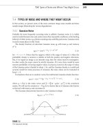
17.4 Quantization 427
50 100 150 200 250 300 350 400 450 500
50
100
150
200
250
300
350
400
450
500
180 190 200 210 220 230
270
280
290
300
310
320
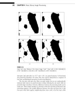
FIGURE 17.2
The original 512 ϫ 512 Lena image (top) with an 8 ϫ 8 block (bottom) identified with black
boundary and with one corner at [209, 297].
428 CHAPTER 17 JPEG and JPEG2000
187 188 189 202 209 175 66 41
191
186 193 209 193 98 40 39
188 187 202 202 144 53 35 37
189 195 206 172 58 47 43 45
197 204 194 106 50 48 42 45
208 204 151 50 41 41 41 53
209 179 68 42 35 36 40 47

200 117 53 41 34 38 39 63
FIGURE 17.3
The 8 ϫ 8 block identified in Fig. 17.2.
915.6 451.3 25.6 212.6 16.1 212.3 7.9 27.3
216.8 19.8 2228.2 225.7 23.0 20.1 6.4 2.0
22.0 277.4 223.8 102.9 45.2 223.7 24.4 25.1
30.1 2.4 19.5 28.6 251.1 232.5 12.3 4.5
5.1 222.1 22.2 21.9 217.4 20.8 23.2 214.5
20.4 20.8 7.5 6.2 29.6 5.7 29.5 219.9
5.3 25.3 22.4 22.4 23.5 22.1 10.0 11.0
0.9 0.7 27.7 9.3 2.7 25.4 26.7 2.5
FIGURE 17.4
DCT of the 8 ϫ 8 block in Fig. 17.3.
values of q[m,n] are restricted to be integers with 1 Յ q[m,n]Յ 255, and they deter-
mine the quantization step for the corresponding coefficient. The quantized coefficient is
given by
qX[m,n]ϭ

X[m,n]
q[m,n]

round
.
A quantization table (or matrix) is required for each image component. How-
ever, a quantization table can be shared by multiple components. For example, in a
luminance-plus-chrominance Y Ϫ Cr Ϫ Cb representation, the two chrominance com-
ponents usually share a common quantization matrix. JPEG quantization tables given in
Annex K of the standard for luminance and components are shown in Fig. 17.5. These
tables were obtained from a series of psychovisual experiments to determine the visibility
thresholds for the DCT basis functions for a 760 ϫ 576 image with chrominance com-

ponents downsampled by 2 in the horizontal direction and at a viewing distance equal
to six times the screen width. On examining the tables, we observe that the quantization
table for the chrominance components has larger values in general implying that the
quantization of the chrominance planes is coarser when compared with the luminance
plane. This is done to exploit the human visual system’s (HVS) relative insensitivity to
chrominance components as compared with luminance components. The tables shown
17.4 Quantization 429
16 11 10 16 24 40 51 61
12 12 14 19 26 58 60 55
14 13 16 24 40 57 69 56
14 17 22 29 51 87 80 62
18 22 37 56 68 109 103 77
24 35 55 64 81 104 113 92
49 64 78 87 103 121 120 101
72 92 95 98 112 100 103 99
17 18 24 47
18 21 26 66
24 26 56
47 66
99 99
99
99
99
99
99
99
99
99
99
99

99
99
99
99
99
99
99
99
99
99
99
99
99
99
99
99
99
99
99
99
99
99
99
99
99
99
99
99
99
99

99
99
99
99
99
99
99
99
99
FIGURE 17.5
Example quantization tables for luminance (left) and chrominance (right) components provided
in the informative sections of the standard.
have been known to offer satisfactory performance, on the average, over a wide variety
of applications and viewing conditions. Hence they have been widely accepted and over
the years have become known as the “default” quantization tables.
Quantization tables can also be constructed by casting the problem as one of optimum
allocation of a given budget of bits based on the coefficient statistics. The general principle
is to estimate the variances of the DCT coefficients and assign more bits to coefficients
with larger variances.
We now examine the quantization of the DCT coefficients given in Fig. 17.4 using
the luminance quantization table in Fig. 17.5(a). Each DCT coefficient is divided by the
corresponding entry in the quantization table, and the result is rounded to yield the array
of quantized DCT coefficients in Fig. 17.6. We observe that a large number of quantized
DCT coefficients are zero, making the array suitable for runlength coding as described in
Section 17.6.Theblock fromthe Lena imagerecovered afterdecoding is shown inFig.17.7.
17.4.2 Quantization Table Design
With lossy compression, the amount of distortion introduced in the image is inversely
related to the number of bits (bit rate) used to encode the image. The higher the rate,
the lower the distortion. Naturally, for a given rate, we would like to incur the minimum
possible distortion. Similarly, for a given distortion level, we would like to encode with

the minimum rate possible. Hence lossy compression techniques are often studied in
terms of their rate-distortion (RD) performance that bounds according to the highest
compression achievable at a given level of distortion they introduce over different bit
rates. The RD performance of JPEG is determined mainly by the quantization tables.
As mentioned before, the standard does not recommend any particular table or set of
tables and leaves their design completely to the user. While the image quality obtained
from the use of the “default” quantization tables described earlier is ver y good, there is a
need to provide flexibility to adjust the image quality by changing the overall bit rate. In
practice, scaled versions of the “default” quantization tables are very commonly used to
vary the quality and compression performance of JPEG. For example, the popular IJPEG
implementation, freely available in the public domain, allows this adjustment through
430 CHAPTER 17 JPEG and JPEG2000
57 41 2 0 0 0 0 0
18 1 216 210000
0 25 2141000
20 0021000
0 21000000
00 00 0000
00 00 0000
00 00 0000
FIGURE 17.6
8 ϫ 8 discrete cosine transform block in Fig. 17.4 after quantization with the luminance quan-
tization table shown in Fig. 17.5.
181 185 196 208 203 159 86 27
191 189 197 203 178 118 58 25
192 193 197 185 136 72 36 33
184 199 195 151 90 48 38 43
185 207 185 110 52 43 49 44
201 198 151 74 32 40 48 38
213 161 92 47 32 35 41 45

216 122 43 32 39 32 36 58
FIGURE 17.7
The block selected from the Lena image recovered after decoding.
the use of quality factor Q for scaling all elements of the quantization table. The scaling
factor is computed as
Scale factor ϭ
⎧
⎪
⎨
⎪
⎩
ϩ
5000
Q
for 1 Յ Q < 50
200 Ϫ 2 ∗Q for 50 Յ Q Յ 99
1 for Q ϭ 100
. (17.1)
Although varying the rate by scaling a base quantization table according to some fixed
scheme is convenient, it is clearly not optimal. Given an image and a bit rate, there exists
a quantization table that provides the “optimal” distortion at the given rate. Clearly, the
“optimal” table would vary with different images and different bit rates and even different
definitions of distortion such as mean square error (MSE) or perceptual distortion. To
get the best performance from JPEG in a given application, custom quantization tables
may need to be designed. Indeed, there has been a lot of work reported in the literature
addressing the issue of quantization table design for JPEG. Broadly speaking, this work
can be classified into three categories. The first deals with explicitly optimizing the RD
performance of JPEG based on statistical mo dels for DCT coefficient distributions. The
second attempts to optimize the visual quality of the reconstructed image at a given
bit rate, given a set of display conditions and a perception model. The third addresses

constraints imposed by applications, such as optimization for printers.
17.4 Quantization 431
An example of the first approach is provided by the work of Ratnakar and Livny [30]
who propose RD-OPT, an efficient algor ithm for constructing quantization tables with
optimal RD performance for a given image. The RD-OPT algorithm uses DCT coefficient
distribution statistics from any given image in a novel way to optimize quantization
tables simultaneously for the entire possible range of compression-quality tradeoffs. The
algorithm is restricted to the MSE-related distortion measures as it exploits the property
that the DCT is a unitary transform, that is, MSE in the pixel domain is the same as MSE
in the DCT domain. The RD-OPT essentially consists of the following three stages:
1. Gather DCT statistics for the given image or set of images. Essentially this step
involves counting how many times the n-th coefficient gets quantized to the value
v when the quantization step size is q and what is the MSE for the n-th coefficient
at this step size.
2. Use statistics collected above to calculate R
n
(q), the rate for the nth coefficient
when the quantization step size is q and the corresponding distortion is D
n
(q), for
each possible q.TherateR
n
(q) is estimated from the corresponding first-order
entropy of the coefficient at the given quantization step size.
3. Compute R(Q) and D(Q), the rate and distortions for a quantization table Q,as
R(Q) ϭ
63

nϭ0
R

n
(Q[n]) and D(Q) ϭ
63

nϭ0
D
n
(Q[n]),
respectively. Use dynamic programming to optimize R(Q) against D(Q).
Optimizing quantization tables with respect to MSE may not be the best strategy
when the end image is to be viewed by a human. A better approach is to match the quan-
tization table to the human visual system HVS model. As mentioned before, the “default”
quantization tables were arrived at in an image independent manner, based on the visi-
bility of the DCT basis functions. Clearly, better performance could be achieved by an
image dependent approach that exploits HVS properties like frequency, contrast, and tex-
ture masking and sensitivity. A number of HVS model based techniques for quantization
table design have been proposed in the literature [3, 18, 41]. Such techniques perform
an analysis of the given image and arrive at a set of thresholds, one for each coefficient,
called the just noticeable distortion (JND) thresholds. The underlying idea being that if
the distortion intro duced is at or just below these thresholds, the reconstructed image
will be perceptually distortion free.
Optimizing quantization tables with respect to MSE may also not be appropriate
when there are constraints on the type of distortion that can be tolerated. For example,
on examining Fig. 17.5, it is clear that the “high-frequency” AC quantization factors, i.e.,
q[m,n] for larger values of m and n, are significantly greater than the DC coefficient
q[0,0] and the “low-frequency” AC quantization factors. There are applications in which
the information of interest in an image may reside in the high-frequency AC coeffi-
cients. For example, in compression of radiographic images [34], the critical diagnostic
432 CHAPTER 17 JPEG and JPEG2000
information is often in the high-frequency components. The size of microcalcification in

mammograms is often so small that a coarse quantization of the higher AC coefficients
will be unacceptable. In such cases, JPEG allows custom tables to be provided in the
bitstreams.
Finally, quantization tables can also be optimized for hard copy devices like printers.
JPEG was designed for compressing images that are to be displayed on devices that use
cathode ray tube that offers a large range of pixel intensities. Hence, when an image
is rendered through a half-tone device [40] like a printer, the image quality could be
far from optimal. Vander Kam and Wong [37] g ive a closed-loop procedure to design
a quantization table that is optimum for a given half-toning and scaling method. The
basic idea behind their algorithm is to code more coarsely frequency components that are
corrupted by half-toning and to code more finely components that are left untouched by
half-toning. Similarly, to take into account the effects of scaling, their design procedure
assigns higher bit rate to the frequency components that correspond to a large gain in
the scaling filter response and lower bit rate to components that are attenuated by the
scaling filter.
17.5 COEFFICIENT-TO-SYMBOL MAPPING AND CODING
The quantizer makes the coding lossy, but it provides the major contribution in com-
pression. However, the nature of the quantized DCT coefficients and the preponderance
of zeros in the array leads to further compression with the use of lossless coding. This
requires that the quantized coefficients be mapped to symbols in such a way that the sym-
bols lend themselves to effective coding. For this purpose, JPEG treats the DC coefficient
and the set of AC coefficients in a different manner. Once the symbols are defined, they
are represented with Huffman coding or arithmetic coding.
In defining symbols for coding, the DCT coefficients are scanned by traversing the
quantized coefficient array i n a zig-zag fashion shown in Fig. 17.8. The zig-zag scan
processes the DCT coefficients in increasing order of spatial frequency. Recall that the
quantized high-frequency coefficients are zero with high probability. Hence scanning in
this order leads to a sequence that contains a large number of trailing zero values and can
be efficiently coded as shown below.
The [0,0]-th element or the quantized DC coefficient is first separated from the

remaining string of 63 AC coefficients,and symbols are defined next as shown in Fig. 17.9.
17.5.1 DC Coefficient Symbols
The DC coefficients in adjacent blocks are highly correlated. This fact is exploited to
differentially code them. Let qX
i
[0,0]and qX
iϪ1
[0,0]denote the quantized DC coefficient
in blocks i and i Ϫ 1. The difference ␦
i
ϭ qX
i
[0,0]Ϫ qX
iϪ1
[0,0] is computed. Assuming
a precision of 8 bits/pixel for each component, it follows that the largest DC coefficient
value (with q[0,0]= 1) is less than 2048, so that values of ␦
i
are in the range [Ϫ2047, 2047].
If Huffman coding is used, then these possible values would require a very large coding
17.5 Coefficient-to-Symbol Mapping and Coding 433
01234567
0
1
2
3
4
5
6
7

FIGURE 17.8
Zig-zag scan procedure.
table. In order to limit the size of the coding table, the values in this range are grouped
into 12 size categories, which are assigned labels 0 through 11. Category k contains 2
k
elements {Ϯ 2
kϪ1
, , Ϯ (2
k
Ϫ 1)}. The difference ␦
i
is mapped to a symbol described by
a pair (category, amplitude). The 12 categories are Huffman coded. To distinguish values
within the same category, extra k bits are used to represent a specific one of the possible
2
k
“amplitudes” of symbols within category k. The amplitude of ␦
i
{2
kϪ1
Յ ␦
i
Յ 2
k
Ϫ 1}
is simply given by its binary representation. On the other hand, the amplitude of ␦
i
{Ϫ2
k
Ϫ 1 Յ ␦

i
ՅϪ2
kϪ1
} is given by the one’s complement of the absolute value |␦
i
| or
simply by the binary representation of ␦
i
ϩ 2
k
Ϫ 1.
17.5.2 Mapping AC Coefficient to Symbols
As observed before, most of the quantized AC coefficients are zero. The zig-zag scanned
string of 63 coefficients contains many consecutive occurrences or“runs of zeros”, making
the quantized AC coefficients suitable for run-length coding (RLC). The symbols in this
case are conveniently defined as [size of run of zeros, nonzero terminating value], which
can then be entropy coded. However, the number of possible values of AC coefficients
is large as is evident from the definition of DCT. For 8-bit pixels, the allowed range of
AC coefficient values is [Ϫ1023,1023]. In view of the large coding tables this entails,
a procedure similar to that discussed above for DC coefficients is used. Categories are
defined for suitable grouped values that can terminate a run. Thus a run/category pair
together with the amplitude within a category is used to define a symbol. The category
definitions and amplitude bits generation use the same procedure as in DC coefficient
difference coding. Thus, a 4-bit category value is concatenated with a 4-bit run length to
get an 8-bit [run/category] symbol. This symbol is then encoded using either Huffman or
434 CHAPTER 17 JPEG and JPEG2000
(a) DC coding
Difference ␦
i
22 [2,22] 01101

Code
(b) AC coding
Terminating
value
Run/
categ.
Code
length
Code Total
bits
Amplitude
bits
0/6 7 1111000 13 010110
0/5 5 11010 10 10010
1/1 4 1100 5 1
0/2 2 01 4 10
1/5 11 11111110110 16 01111
0/3 3 100 6 010
0/2 2 01 4 10
2/1 5 11100 6 0
0/1 2 00 3 0
3/3 12 111111110101 15 100
1/1 4 1100 5 1
5/1 7 1111010 8 1
5/1 7 1111010 8 0
41
18
1
2
216

25
2
21
21
4
21
1
21
EOB
EOB 4
112
1010 4 2
Total bits for block
Rate 5 112/64 5 1.75 bits per pixel
[Category, Amplitude]
FIGURE 17.9
(a) Coding of DC coefficient with value 57, assuming that the previous block has a DC coefficient
of value 59; (b) Coding of AC coefficients.
arithmetic coding. T here are two special cases that arise when coding the [run/category]
symbol. First, since the run value is restricted to 15, the symbol (15/0) is used to denote
fifteen zeroes followed by a zero. A number of such symbols can be cascaded to specify
larger runs. Second, if after a nonzero AC coefficient, all the remaining coefficients are
zero, then a special symbol (0/0) denoting an end-of-block (EOB) is encoded. Fig. 17.9
continues our example and shows the sequence of symbols generated for coding the
quantized DCT block in the example show n in Fig. 17.6.
17.5.3 Entropy Coding
The symbols defined for DC and AC coefficients are entropy coded using mostly Huffman
coding or, optionally and infrequently, arithmetic coding based on the probability esti-
mates of the symbols. Huffman coding is a method of VLC in which shorter code words
are assigned to the more frequently occurring symbols in order to achieve an average

symbol code word length that is as close to the symbol source entropy as possible.
17.6 Image Data Format and Components 435
Huffman coding is optimal (meets the entropy bound) only when the symbol proba-
bilities are integral powers of 1/2. The technique of arithmetic coding [42] provides a
solution to attaining the theoretical bound of the source entropy. The baseline
implementation of the JPEG standard uses Huffman coding only.
If Huffman coding is used, then Huffman tables,up to a maximum of eight in number,
are specified in the bitstream. The tables constructed should not contain code words that
(a) are more than 16 bits long or (b) consist of all ones. Recommended tables are listed in
annex K of the standard. If these tables are applied to the output of the quantizer shown
in the first two columns of Fig. 17.9, then the algorithm produces output bits shown in
the following columns of the figure. The procedures for specification and generation of
the Huffman tables are identical to the ones used in the lossless standard [25].
17.6 IMAGE DATA FORMAT AND COMPONENTS
The JPEG standard is intended for the compression of both grayscale and color images.
In a grayscale image, there is a single “luminance” component. However, a color image
is represented w ith multiple components, and the JPEG standard sets stipulations on the
allowed number of components and data formats. The standard permits a maximum
of 255 color components which are rectangular arrays of pixel values represented with
8- to 12-bit precision. For each color component, the largest dimension supported in
either the horizontal or the vertical direction is 2
16
ϭ 65,536.
All color component arrays do not necessarily have the same dimensions. Assume that
an image contains K color components denoted by C
n
, n ϭ 1,2, ,K . Let the horizontal
and vertical dimensions of the n-th component be equal to X
n
and Y

n
, respectively. Define
dimensions X
max
,Y
max
, and X
min
,Y
min
as
X
max
ϭ max
K
nϭ1
{X
n
}, Y
max
ϭ max
K
nϭ1
{Y
n
}
and
X
min
ϭ min

K
nϭ1
{X
n
}, Y
min
ϭ min
K
nϭ1
{Y
n
}.
Each color component C
n
, n ϭ 1,2, ,K , is associated with relative horizontal and
vertical sampling factors, denoted by H
n
and V
n
respectively, where
H
n
ϭ
X
n
X
min
, V
n
ϭ

Y
n
Y
min
.
The standard restricts the possible values of H
n
and V
n
to the set of four integers 1,2,3,4.
The largest values of relative sampling factors are given by H
max
ϭ max{H
n
}and V
max
ϭ
max{V
n
}.
According to the JFIF, the color information is specified by [X
max
, Y
max
, H
n
and
V
n
, n ϭ 1, 2, ,K , H

max
, V
max
]. The horizontal dimensions of the components are
436 CHAPTER 17 JPEG and JPEG2000
computed by the decoder as
X
n
ϭ X
max
ϫ
H
n
H
max
.
Example 1: Consider a raw image in a luminance-plus-chrominance representation
consisting of K ϭ 3 components, C
1
ϭ Y , C
2
ϭ Cr, and C
3
ϭ Cb. Let the dimensions
of the luminance matrix (Y )beX
1
ϭ 720 and Y
1
ϭ 480, and the dimensions of the two
chrominance matrices (Cr and Cb)beX

2
ϭ X
3
ϭ 360 and Y
2
ϭ Y
3
ϭ 240. In this case,
X
max
ϭ 720 and Y
max
ϭ 480, and X
min
ϭ 360 and Y
min
ϭ 240. The relative sampling
factors are H
1
ϭ V
1
ϭ 2 and H
2
ϭ V
2
ϭ H
3
ϭ V
3
ϭ 1.

When images have multiplecomponents, the standard specifies formats for organizing
the data for the purpose of storage. In storing components, the standard provides the
option of using either interleaved or noninterleaved formats. Processing and storage
efficiency is aided, however, by interleaving the components where the data is read in
a single scan. Interleaving is performed by defining a data unit for lossy coding as a
single block of 8 ϫ 8 pixels in each color component. This definition can be used to
partition the n-th color component C
n
, n ϭ 1, 2, ,K , into rectangular blocks, each
of which contains H
n
ϫ V
n
data units. A minimum coded unit (MCU) is then defined as
the smallest interleaved collection of data units obtained by successively picking H
n
ϫ V
n
data units from the n-th color component. Certain restrictions are imposed on the data
in order to be stored in the interleaved format:
■ The number of interleaved components should not exceed four;
■ An MCU should contain no more than ten data units, i.e.,
K

nϭ1
H
n
V
n
Յ 10.

If the above restrictions are not met, then the data is stored in a noninterleaved format,
where each component is processed in successive scans.
Example 2: Let us consider the case of storage of the Y , Cr, Cb components in
Example 1. The luminance component contains 90 ϫ 60 data units, and each of the
two chrominance components contains 45 ϫ 30 data units. Figure 17.10 shows both
a noninterleaved and an interleaved arrangement of the data for K ϭ 3 components,
C
1
ϭ Y , C
2
ϭ Cr, and C
3
ϭ Cb, with H
1
ϭ V
1
ϭ 2 and H
2
ϭ V
2
ϭ H
3
ϭ V
3
ϭ 1. The
MCU in this case contains six data units, consisting of H
1
ϫ V
1
ϭ 4 data units of the Y

component and H
2
ϫ V
2
ϭ H
3
ϫ V
3
ϭ 1eachoftheCr and Cb components.
17.7 ALTERNATIVE MODES OF OPERATION
What has been described thus far in this chapter represents the JPEG sequential DCT
mode. The sequential DCT mode is the most commonly used mode of operation of
17.7 Alternative Modes of Operation 437
Cr1:1 Cb1:1
Y2:2
Y1:2
Y2:1
Y1:1
Y60:90
Cb30:45Cr30:45
Cr component
data units
Cb component
data units
Noninterleaved format:
Interleaved format:
Y component
data units
Cr1:1 Cr1:2 Cr30:45
Y1:1 Y1:2 Y1:90 Y2:1 Y2:2 Y60:89 Y60:90 Cb1:1 Cb1:2 Cb30:45

Y60:89
Y59:89 Y 59:90
Y1:1 Y1:2 Y2:1 Y2:2 Cr1:1 Cb1:1 Y1:3 Y1:4 Y2:3 Y2:4 Cr1:2 Cr1:2
Y59:89 Y59:90 Y60:89 Y60:90 Cr30:45 Cb30:45
MCU-1 MCU-2
MCU-1350
FIGURE 17.10
Organizations of the data units in the Y , Cr, Cb components into noninterleaved and interleaved
formats.
JPEG and is required to be supported by any baseline implementation of the standard.
However, in addition to the sequential DCT mode, JPEG also defines a progressive DCT
mode, sequential lossless mode, and a hierarchical mode.InFigure 17.11 we show how
the different modes can be used. For example, the hierarchical mode could be used in
conjunction with any of the other modes as shown in the figure. In the lossless mode,JPEG
uses an entirely different algorithm based on predictive coding [25]. In this section we
restrict our attention to lossy compression and describe in greater detail the DCT-based
progressive and hierarchical modes of operation.
17.7.1 Progressive Mode
In some applications it may be advantageous to transmit an image in multiple passes,
such that after each pass an increasingly accurate approximation to the final image can
be constructed at the receiver. In the first pass, ver y few bits are transmitted and the
reconstructed image is equivalent to one obtained w ith a very low quality setting. Each of
the subsequent passes contain an increasing number of bits which are used to refine the
quality of the reconstructed image. The total number of bits transmitted is roughly the
same as would be needed to transmit the final image by the sequential DCT mode. One
example of an application which would benefit from progressive transmission is provided
438 CHAPTER 17 JPEG and JPEG2000
Sequential
mode
Hierarchical

mode
Progressive
mode
Spectral
selection
Successive
approximation
FIGURE 17.11
JPEG modes of operation.
by Internet image access, where a user might want to start examining the contents of the
entire page without waiting for each and every image contained in the page to be fully and
sequentially downloaded. Other examples include remote browsing of image databases,
tele-medicine, and network-centric computing in general. JPEG contains a progressive
mode of coding that is well suited to such applications. The disadvantage of progressive
transmission, of course, is that the image has to be decoded a multiple number of times,
and its use only makes sense if the decoder is faster than the communication link.
In the progressive mode, the DCT coefficients are encoded in a series of scans. JPEG
defines two ways for doing this: spectral selection and successive approximation. In the
spectral selection mode, DCT coefficients are assigned to different groups according to
their position in the DCT block, and during each pass, the DCT coefficients belonging to
a single group are transmitted. For example, consider the following grouping of the 64
DCT coefficients numbered from 0 to 63 in the zig-zag scan order,
{0},{1, 2, 3},{4, 5, 6, 7}, {8, ,63}.
Here, only the DC coefficient is encoded in the first scan. This is a requirement imposed
by the standard. In the progressive DCT mode, DC coefficients are always sent in a
separate scan. The second scan of the example codes the first three AC coefficients in
zig-zag order, the third scan encodes the next four AC coefficients, and the fourth and
the last scan encodes the remaining coefficients. JPEG provides the syntax for specifying
the starting coefficient number and the final coefficient number being encoded in a
particular scan. This limits a group of coefficients being encoded in any given scan to

being successive in the zig-zag order. The first few DCT coefficients are often sufficient
to give a reasonable rendition of the image. In fact, just the DC coefficient can serve to
essentially identify the contents of an image, although the reconstructed image contains
17.7 Alternative Modes of Operation 439
severe blocking ar tifacts. It should be noted that after all the scans are decoded, the final
image quality is the same as that obtained by a s equential mode of operation. The bit
rate, however, can be different as the entropy coding procedures for the progressive mode
are different as described later in this section.
In successive approximation coding, the DCT coefficients are sent in successive scans
with increasing level of precision. The DC coefficient, however, is sent in the first scan
with full precision, just as in the case of spectral selection coding. The AC coefficients
are sent bit plane by bit plane, starting from the most significant bit plane to the least
significant bit plane.
The entropy coding techniques used in the progressive mode are slightly different
from those used in the sequential mode. Since the DC coefficient is always sent as a
separate scan, the Huffman and arithmetic coding procedures used remain the same
as those in the sequential mode. However, coding of the AC coefficients is done a bit
differently. In spectral selection coding (without selective refinement) and in the first
stage of successive approximation coding, a new set of symbols is defined to indicate runs
of EOB codes. Recall that in the sequential mode the EOB code indicates that the rest of
the block contains zero coefficients. With spectral selection, each scan contains only a few
AC coefficients and the probability of encountering EOB is significantly higher. Similarly,
in successive approximation coding, each block consists of reduced precision coefficients,
leading again to a large number of EOB symbols being encoded. Hence, to exploit this
fact and achieve further reduction in bit rate, JPEG defines an additional set of fifteen
symbols, EOB
n
, each representing a run of 2
n
EOB codes. After each EOB

i
run-length
code, extra i bits are appended to specify the exact run-length.
It should be noted that the two progressive modes, spectral selection and successive
refinement,can be combined to give successive approximation in each spectral band being
encoded. This results in quite a complex codec, which to our knowledge is rarely used.
It is possible to transcode between progressive JPEG and sequential JPEG without any
loss in quality and approximately maintaining the same bit rate. Spectral selection results
in bit rates slightly higher than the sequential mode, whereas successive approximation
often results in lower bit rates. The differences however are small.
Despite the advantages of progressive transmission, there have not been many imple-
mentations of progressive JPEG codecs. There has been some interest in them due to the
proliferation of images on the Internet.
17.7.2 Hierarchical Mode
The hierarchical mode defines another form of progressive transmission where the image
is decomposed into a pyramidal structure of increasing resolution. The top-most layer in
the pyramid represents the image at the lowest resolution, and the base of the pyramid
represents the image at full resolution. There is a doubling of resolutions both in the
horizontal and vertical dimensions, between successive levels in the pyramid. Hierarchical
coding is useful when an image could be displayed at different resolutions in units such
as handheld devices, computer monitors of varying resolutions, and high-resolution
printers. In such a scenario, a multiresolution representation allows the transmission
440 CHAPTER 17 JPEG and JPEG2000
-
Downsampling
filter
Upsampling filter
with bilinear
interpolation
Difference

image
Image at level k
Image at level
k
- 1
FIGURE 17.12
JPEG hierarchical mode.
of the appropriate layer to each requesting device, thereby making full use of available
bandwidth.
In the JPEG hierarchical mode, each image component is encoded a s a sequence of
frames. The lowest resolution frame (level 1) is encoded using one of the sequential or
progressive modes. The remaining levels are encoded differentially. That is, an estimate I
Ј
i
of the image, I
i
, at the i
Ј
th level (i Ն 2) is first formed by upsampling the low-resolution
image I
iϪ1
from the layer immediately above. Then the difference between I
Ј
i
and I
i
is
encoded using modifications of the DCT-based modes or the lossless mode. If lossless
mode is used to code each refinement, then the final reconstruction using all layers is
lossless. The upsampling filter used is a bilinear interpolating filter that is specified by the

standard and cannot be specified by the user. Starting from the high-resolution image,
successive low-resolution images are created essentially by downsampling by two in each
direction. The exact downsampling filter to be used is not specified but the standard
cautions that the downsampling filter used be consistent with the fixed upsampling filter.
Note that the decoder does not need to know what downsampling filter was used in order
to decode a bitstream. Figure 17.12 depicts the sequence of operations performed at each
level of the hierarchy.
Since the differential frames are already signed values, they are not level-shifted prior
to forward discrete cosine transform (FDCT). Also, the DC coefficient is coded directly
rather than differentially. Other than these two features, the Huffman coding model in
the prog ressive mode is the same as that used in the sequential mode. Arithmetic coding
is, however, done a bit differently with conditioning states based on the use of differences
with the pixel to the left as well as the one above. For details the user is referred to [28].
17.8 JPEG Part 3 441
17.8 JPEG PART 3
JPEG has made some recent extensions to the original standard described in [11]. These
extensions are collectively known as JPEG Part 3. The most impor tant elements of JPEG
part 3 are variable quantization and tiling, as described in more detail below.
17.8.1 Variable Quantization
One of the main limitations of the original JPEG standard was the fact that visible
artifacts can often appear in the decompressed image at moderate to high compression
ratios. This is especially true for parts of the image containing graphics, text, or some
synthesized components. Artifacts are also common in smooth regions and in image
blocks containing a single dominant edge. We consider compression of a 24 bits/pixel
color version of the Lena image. In Fig. 17.13 we show the reconstructed Lena image
with different compression ratios. At 24 to 1 compression we see few artifacts. However,
as the compression ratio is increased to 96 to 1, noticeable artifacts begin to appear.
Especially annoying is the “blocking artifact” in smooth regions of the image.
One approach to deal with this problem is to change the “coarseness” of quantization
as a function of image characteristics in the block being compressed. The latest extension

of the JPEG standard, called JPEG Part 3, allows rescaling of quantization matrix Q on a
block by block basis, thereby potentially changing the manner in which quantization is
performed for each block. The scaling operation is not done on the DC coefficient Y [0,0]
which is quantized in the same manner as in the baseline JPEG. The remaining 63 AC
coefficients, Y [u, v], are quantized as follows:
ˆ
Y [u,v]ϭ

Y [u,v]ϫ 16
Q[u,v]ϫ QScale

,
where QScale is a parameter that can take on values from 1 to 112, with a default value of
16. For the decoder to correctly recover the quantized AC coefficients, it needs to know
the value of QScale used by the encoding process. The standard specifies the exact syntax
by which the encoder can specify change in QScale values. If no such change is signaled,
then the decoder continues using the QScale value that is in current use. The overhead
incurred in signaling a change in the scale factor is approximately 15 bits depending on
the Huffman table being employed.
It should be noted that the standard only specifies the syntax by means of which the
encoding process can signal changes made to the QScale value. It does not specify how
the encoder may determine if a change in QScale is desired and what the new value of
QScale should be. Typical methods for variable quantization proposed in the literature
use the fact that the HVS is less sensitive to quantization errors in highly active regions of
the image. Quantization errors are frequently more perceptible in blocks that are smooth
or contain a single dominant edge. Hence, prior to quantization, a few simple features for
each block are computed. These features are used to classify the block as either smooth,
edge, or texture, and so forth. On the basis of this classification as well as a simple activity
measure computed for the block, a QScale value is computed.
442 CHAPTER 17 JPEG and JPEG2000

FIGURE 17.13
Lena image at 24 to 1 (top) and 96 to 1 (bottom) compression ratios.
17.8 JPEG Part 3 443
For example, Konstantinides and Tretter [21] give an algorithm for computing QScale
factors for improving text quality on compound documents. They compute an activity
measure M
i
for each image block as a function of the DCT coefficients as follows:
M
i
ϭ
1
64
⎡
⎣
log
2
|Y
i
[0,0]Ϫ Y
iϪ1
[0,0]|ϩ

j,k
log
2
|Y
i
[j,k]|
⎤

⎦
. (17.2)
The QScale value for the block is then computed as
QScale
i
ϭ
⎧
⎪
⎨
⎪
⎩
a ϫ M
i
ϩ bif2 > a ϫ M
i
ϩ b Ն 0.4
0.4 a ϫ M
i
ϩ b Ն 0.4
2 a ϫ M
i
ϩ b > 2.
(17.3)
The technique is only designed to detect text regions and will quantize high-activity tex-
tured regions in the image part at the same scale as text regions. Clearly, this is not optimal
as high-activity textured regions can be quantized very coarsely leading to improved com-
pression. In addition, the technique does not discriminate smooth blocks where artifacts
are often the first to appear.
Algorithms for variable quantization that perform a more extensive classification have
been proposed for video coding but nevertheless are also applicable to still image coding .

One such technique has been proposed by Chun et al. [10] who classify blocks as being
either smooth, edge, or texture, based on several parameters defined in the DCT domain
as shown below:
E
h
: horizontal energy E
v
: vertical energy E
d
: diagonal energy
E
a
: avg (E
h
,E
v
,E
d
) E
m
: min(E
h
,E
v
,E
d
) E
M
: max(E
h

,E
v
,E
d
)
E
m/M
: ratio of E
m
and E
M
.
E
a
represents the average high-frequency energy of the block, and is used to distinguish
between low-activity blocks and high-activity blocks. Low-activity (smooth) blocks sat-
isfy the relationship, E
a
Յ T
1
,whereT
1
is a low-valued threshold. High-activity blocks
are further classified into texture blocks and edge blocks. Texture blocks are detected
under the assumption that they have relatively uniform energy distribution in compari-
son with edge blocks. Specifically, a block is deemed to be a texture block if it satisfies the
conditions: E
a
> T
1

, E
min
> T
2
, and E
m/M
> T
3
,whereT
1
,T
2
, and T
3
are experimentally
determined constants. All blocks which fail to satisfy the smoothness and texture tests
are classified as edge blocks.
17.8.2 Tiling
JPEG Part 3 defines a tiling capability whereby an image is subdivi ded into blocks or tiles,
each coded independently. Tiling facilitates the following features:
■ Display of an image region on a given screen size;
■ Fast access to image subregions;
444 CHAPTER 17 JPEG and JPEG2000
0
1
2
345
679
Tile
1

Tile
2
Tile 3
Tile
1
Tile
2
Tile 3
(a) (b)
(c)
FIGURE 17.14
Different types of tilings allowed in JPEG Part 3: (a) simple; (b) composite; and (c) pyramidal.
■ Region of interest refinement;
■
Protection of large images from copying by giving access to only a part of it.
As shown in Fig. 17.14, the different types of tiling allowed by JPEG are as follows:
■ Simple tiling: This form of tiling is essentially used for dividing a large image
into multiple sub-images which are of the same size (except for edges) and are
nonoverlapping. In this mode, all tiles are required to have the same sampling
factors and components. Other parameters like quantization tables and Huffman
tables are allowed to change from tile to tile.
■ Composite tiling: This allows multiple resolutions on a single image display plane.
Tiles can overlap within a plane.
■
Pyramidal tiling: This is used for storing multiple resolutions of an image. Simple
tiling as described above is used in each resolution. Tiles are stored in raster order,
left to right, top to bottom, and low resolution to high resolution.
17.9 The JPEG2000 Standard 445
Another Part 3 extension is selective refinement. This feature per mits a scan in a
progressive mode, or a specific level of a hierarchical sequence, to cover only part of

the total image area. Selective refinement could be useful, for example, in telemedicine
applications where a radiologist could request refinements to specific areas of interest in
the image.
17.9 THE JPEG2000 STANDARD
The JPEG standard has proved to be a tremendous success over the past decade in
many digital imaging applications. However, as the needs of multimedia and imaging
applications evolved in areas such as medical imaging, reconnaissance, the Internet, and
mobile imaging, it became evident that the JPEG standard suffered from shortcomings
in compression efficiency and progressive decoding. This led the JPEG committee to
launch an effort in late 1996 and early 1997 to create a new image compression standard.
The intent was to provide a method that would support a range of features in a single
compressed bitstream for different types of still images such as bilevel, gray level, color,
multicomponent—in particular multispectral—or other types of imagery.A call for tech-
nical contributions was issued in March 1997. Twenty-four proposals were submitted for
consideration by the committee in November 1997. Their evaluation led to the selection
of a wavelet-based coding architecture as the backbone for the emerging coding system.
The initial solution, inspired by the wavelet trellis-coded quantization (WTCQ) algo-
rithm [32] based on combining wavelets and trellis-coded quantization (TCQ) [6, 23],
has been refined via a series of core experiments over the ensuing three years. The initia-
tive resulted in the ISO 15444/ITU-T Recommendation T.8000 known as the JPEG2000
standard. It comprises six parts that are either complete or nearly complete at the time
of writing this chapter, together with four new parts that are under development. The
status of the parts is available at the official website [19].
Part 1, in the spirit of the JPEG baseline system, specifies the core compression system
together with a minimal file format [13]. JPEG2000 Part 1 addresses some limitations of
existing standards by supporting the following features:
■
Lossless and lossy compression of continuous-tone and bilevel images with reduced
distortion and superior subjective performance.
■

Progressive transmission and decoding based on resolution scalability by pixel
accuracy (i.e., based on quality or signal-to-noise (SNR) scalability). The bytes
extracted are identical to those that would be generated if the image had been
encoded targeting the desired resolution or quality,the latter being directly available
without the need for decoding and re-encoding.
■ Random access to spatial reg ions (or regions of interest) as well as to components.
Each region can be accessed at a variety of resolutions and qualities.
■ Robustness to bit errors (e.g., for mobile image communication).
446 CHAPTER 17 JPEG and JPEG2000
■ Encoding capability for sequential scan, thereby avoiding the need to buffer the
entire image to be encoded. This is especially useful when manipulating images of
very large dimensions such as those encountered in reconnaissance (satellite and
radar) images.
Some of the above features are supported to a limited extent in the JPEG standard. For
instance, as described earlier, the JPEG standard has four modes of operation: sequential,
progressive, hierarchical, and lossless. These modes use different techniques for encod-
ing (e.g., the lossless compression mode relies on predictive coding, whereas the lossy
compression modes rely on the DCT). One drawback is that if the JPEG lossless mode
is used, then lossy decompression using the lossless encoded bitstream is not possible.
One major advantage of JPEG2000 is that these four operation modes are integrated in
it in a “compress once, decompress many” par adigm, with superior RD and subjective
performance over a large range of RD operating points.
Part 2 specifies extensions to the core compression system and a more complete file
format [14]. These extensions address additional coding features such as generalized
and variable quantization offsets, TCQ, visual masking, and multiple component trans-
formations. In addition it includes features for image editing such as cropping in the
compressed domain or mirroring and flipping in a partially-compressed domain.
Parts 3, 4, and 5 provide a specification for motion JPEG 2000, conformance testing,
and a description of a reference software implementation, respectively [15–17]. Four
parts, numbered 8–11, are still under development at the time of writing. Part 8 deals with

security aspects, Part 9 specifies an interactive protocol and an application programming
interface for accessing JPEG2000 compressed images and files via a network, Part 10 deals
with volumetric imaging, and Part 11 specifies the tools for wireless imaging.
The remainder of this chapter provides a brief overview of JPEG2000 Part 1 and
outlines the main extensions provided in Part 2. The JPEG2000 standard embeds efficient
lossy, near-lossless and lossless representations within the same stream. However, while
some coding tools (e.g ., color transformations, discrete wavelet transfor ms) can be used
both for lossy and lossless coding, others can be used for lossy coding only. This led to the
specification of two coding paths or options referred to as the reversible (embedding lossy
and lossless representations) and irreversible (for lossy coding only) paths with common
and path-specific building blocks. This chapter presents the main components of the
two coding paths which can be used for lossy coding. Discussion of the components
specific to JPEG2000 lossless coding can be found in [25], and a detailed description of
the JPEG2000 coding tools and system can be found in [36]. Tutorials and overviews are
presented in [9, 29, 33].
17.10 JPEG2000 PART 1: CODING ARCHITECTURE
The coding architecture comprises two paths, the irreversible and the reversible paths
shown in Fig. 17.15. Both paths can be used for lossy coding by truncating the compressed
codestream at the desired bit rate. The input image may comprise one or more (up to
16, 384) signed or unsigned components to accommodate various forms of imagery,
17.10 JPEG2000 Part 1: Coding Architecture 447
Level
offset
Irreversible
color
transform
Reversible
DWT
Reversible
color

transform
Irreversible
DWT
Deadzone
quantizer
Ranging
Regions
of
interest
Block
coder
FIGURE 17.15
Main building blocks of the JPEG2000 coder. The path with boxes in dotted lines corresponds
to the JPEG2000 lossless coding mode [25].
including multispectral imagery. The various components may have different bit depth,
resolution, and sign specifications.
17.10.1 Preprocessing: Tiling, Level Offset, and Color Transforms
The first steps in both paths are optional and can be regarded as preprocessing steps.
The image is first, optionally, partitioned into rectangular and nonoverlapping tiles of
equal size. If the sample values are unsigned and represented with B bits, an offset of
Ϫ2
BϪ1
is added leading to a signed representation in the range [Ϫ2
BϪ1
,2
BϪ1
] that is
symmetrically dist ributed about 0. The color component samples may be converted into
luminance and color difference components via an irreversible color transform (ICT)
or a reversible color transform (RCT) in the irreversible or reversible paths, respectively.

448 CHAPTER 17 JPEG and JPEG2000
The ICT is identical to the conversion from RGB to YC
b
C
r
,
⎡
⎢
⎣
Y
C
b
C
r
⎤
⎥
⎦
ϭ
⎡
⎢
⎣
0.299 0.587 0.114
Ϫ0.169 Ϫ0.331 0.500
0.500 Ϫ0.419 Ϫ0.081
⎤
⎥
⎦
⎡
⎢
⎣

R
G
B
⎤
⎥
⎦
,
and can be used for lossy coding only. The RCT is a reversible integer-to-integer transform
that approximates the ICT. This color transform is required for lossless coding [25].The
RCT can also be used for lossy coding, thereby allowing the embedding of both a lossy
and lossless representation of the image in a single codestream.
17.10.2 Discrete Wavelet Transform (DWT)
After tiling, each tile component is decomposed with a forward discrete wavelet transform
(DWT) into a set of L ϭ 2
l
resolution levels using a dyadic decomposition. A detailed
and complete presentation of the theory and implementation of filter banks and wavelets
is beyond the scope of this chapter. The reader is referred to Chapter 6 [26] and to [38]
for additional insight on these issues.
The forward DWT is based on separable wavelet filters and can be irreversible or
reversible. The transforms are then referred to as reversible discrete wavelet transform
(RDWT) and irreversible discrete wavelet transform (IDWT). As for the color transform,
lossy coding can make use of both the IDWT and the RDWT. In the case of RDWT, the
codestream is t runcated to reach a given bit rate. The use of the RDWT allows for both
lossless and lossy compression to be embedded in a single compressed codestream. In
contrast, lossless coding restricts us to the use of only RDWT.
The default RDWT is based on the spline 5/3 wavelet transform first introduced
in [22]. The RDWT filtering kernel is presented elsewhere [25] in this handbook. The
default irreversible transform, IDWT, is implemented with the Daubechies 9/7wavelet
kernel [4]. The coefficients of the analysis and synthesis filters are given in Table 17.1.

Note however that, in JPEG2000 Part 2, other filtering kernels specified by the user can
be used to decompose the image.
TABLE 17.1 Indirect discrete wavelet transform analysis and synthesis filters coefficients.
Index Lowpass analysis Highpass analysis Lowpass synthesis Highpass synthesis
filter coefficient filter coefficient filter coefficient filter coefficient
0 0.602949018236360 1.115087052457000 1.115087052457000 0.602949018236360
ϩ/Ϫ1 0.266864118442875 Ϫ0.591271763114250 0.591271763114250 Ϫ0.266864118442875
ϩ/Ϫ2 Ϫ0.078223266528990 Ϫ0.057543526228500 Ϫ0.057543526228500 Ϫ0.078223266528990
ϩ/Ϫ3 Ϫ0.016864118442875 0.091271763114250 Ϫ0.091271763114250 0.016864118442875
ϩ/Ϫ4 ϩ0.026748757410810 0.026748757410810
17.10 JPEG2000 Part 1: Coding Architecture 449
These filtering kernels are of odd length. Their implementation at the boundary of
the image or subbands requires a sy mmetric signal extension. Two filtering modes are
possible: convolution- and lifting-based [26].
17.10.3 Quantization and Inverse Quantization
JPEG2000 adopts a scalar quantization strategy, similar to that in the JPEG baseline
system. One notable difference is in the use of a central deadzone quantizer. A detailed
description of the procedure can be found in [36]. This section provides only an outline
of the algorithm. In Part 1, the subband samples are quantized with a deadzone scalar
quantizer with a central interval that is twice the quantization step size. The quantization
of y
i
(n) is given by
ˆy
i
(n) ϭ sign(y
i
(n))
|y
i

(n)|
⌬
i
, (17.4)
where ⌬
i
is the quantization step size in the subband i. The parameter ⌬
i
is chosen so
that ⌬
i
ϭ⌬

1
G
i
,whereG
i
is the squared norm of the DWT synthesis basis vectors for
subband i and ⌬ is a parameter to be adjusted to meet g iven RD constraints. The step
size ⌬
i
is represented with two bytes, and consists of a 11-bit mantissa ␮
i
and a 5-bit
exponent ⑀
i
:
⌬
i

ϭ 2
R
i
Ϫ⑀
i

1 ϩ
␮
i
2
11

, (17.5)
where R
i
is the number of bits corresponding to the nominal dynamic range of the
coefficients in subband i. In the reversible path, the step size ⌬
i
is set to 1 by choosing
␮
i
ϭ 0 and ⑀
i
ϭ R
i
.
The nominal dynamic range in subband i depends on the number of bits used to
represent the original tile component and on the wavelet transform used.
The choice of a deadzone that is twice the quantization step size allows for an optimal
bitstream embedded structure, i.e., for SNR scalability. The decoder can, by decoding up

to any truncation point, reconstruct an image identical to what would have been obtained
if encoded at the corresponding target bit rate. All image resolutions and qualities are
directly available from a single compressed stream (also called codestream) without the
need for decoding and re-encoding the existing codestream. In Part 2, the size of the
deadzone can have different values in the different subbands.
Two modes have been specified for signaling the quantization parameters: expounded
and derived. In the expounded mode, the pair of values (⑀
i
,␮
i
) for each subband are
explicitly tr ansmitted. In the derived mode, codestream markers quantization default
and quantization coefficient supply step size parameters only for the lowest frequency
subband. The quantization parameters for other subbands i are then derived according to
(⑀
i
,␮
i
) ϭ (⑀
0
ϩ l
i
Ϫ L,␮
0
), (17.6)
where L is the total number of wavelet decomposition levels and l
i
is the number of levels
required to generate the subband i.
450 CHAPTER 17 JPEG and JPEG2000

The inverse quantization a llows for a reconstruction bias from the quantizer
midpoint for nonzero indices to accommodate s kewed probability distributions of
wavelet coefficients. The reconstructed values are thus computed as
˜y
i
ϭ
⎧
⎪
⎨
⎪
⎩
(ˆy
i
ϩ ␥)⌬
i
2
M
i
ϪN
i
if ˆy
i
> 0,
(ˆy
i
Ϫ ␥)⌬
i
2
M
i

ϪN
i
if ˆy
i
< 0,
0 otherwise.
(17.7)
Here ␥ is a parameter which controls the reconstruction bias; a value of ␥ ϭ 0.5
results in midpoint reconstruction. The term M
i
denotes the maximum number of bits
for a quantizer index in subband i. N
i
represents the number of bits to be decoded in the
case where the embedded bitstream is truncated prior to decoding.
17.10.4 Precincts and Code-blocks
Each subband, after quantization, is divi ded into nonoverlapping rectangular blocks,
called code-blocks, of equal size. The dimensions of the code-blocks are powers of 2 (e.g.,
of size 16 ϫ 16 or 32 ϫ 32), and the total number of coefficients in a code-block should
not exceed 4096. The code-blocks formed by the quantizer indexes corresponding to the
quantized wavelet coefficients constitute the input to the entropy coder. Collections of
spatially consistent code-blocks taken from each subband at each resolution level are
called precincts and will form a packet partition in the bitstream structure. The purpose
of precincts is to enable spatially progressive bitstreams. This point is further elaborated
in Section 17.10.6.
17.10.5 Entropy Coding
The JPEG2000 entropy coding technique is based on the EBCOT (Embedded Block Cod-
ing with Optimal Truncation) algorithm [35]. Each code-block B
i
is enco ded separately,

bit plane by bit plane, starting with the most significant bit plane (MSB) with a nonzero
element and progressing towards the least significant bit plane. The data in each bit plane
is scanned along the stripe pattern shown in Fig. 17.16 (with a stripe heig ht of 4 sam-
ples) and encoded in three passes. Each pass collects contextual information that first
helps decide which primitives to encode. The primitives are then provided to a context-
dependent arithmetic coder. The bit plane encoding procedure is well suited for creating
an embedded bitstream. Note that the approach does not exploit interscale dependencies.
This potential loss in compression efficiency is compensated by beneficial features such
as spatial random access, geometric manipulations in the compression domain, and error
resilience.
17.10.5.1 Context Formation
Let s
i
[k] ϭ s
i
[k
1
,k
2
] be the subband sample belonging to the block B
i
at the horizontal
and vertical positions k
1
and k
2
.Let␹
i
[k]∈{Ϫ1,1} denote the sign of s
i

[k] and ␯
i
[k] ϭ
|s
i
[k]|
␦
␤
i
, the amplitude of the quantized samples represented with M
i
bits, where ␦
␤
i
is the
17.10 JPEG2000 Part 1: Coding Architecture 451
Stripe
Code–block width
FIGURE 17.16
Stripe bit plane scanning pattern.
v
h
d
FIGURE 17.17
Neighbors involved in the context formation.
quantization step of the subband ␤
i
containing the block B
i
.Let␯

b
i
[k] be the bth bit of
the binary representation of ␯
i
[k].
A sample s
i
[k] is said to be nonsignificant (␴(s
i
[k]) ϭ 0) if the first nonzero bit ␯
b
i
[k]
of ␯
i
[k] is yet to be encountered. The statistical dependencies between neighboring
samples are captured via the formation of contexts which depend upon the significance
state variable ␴(s
i
[k]) associated with the eight-connect neighbors depicted in Fig. 17.17.
These contexts are grouped in the following categories:
■ h : number of significant horizontal neighbors, 0 Յ h Յ 2;
■ v : number of significant vertical neighbors, 0 Յ v Յ 2;
■ d : number of significant diagonal neighbors, 0 Յ d Յ 4.
Neighbors which lie beyond the code-block boundary are considered to be nonsignificant
to avoid dependence between code-blocks.