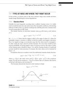
12.2 Weighted Median Smoothers and Filters 273
decomposition of x amounts to decomposing this vector into 2M binary vectors
x
ϪMϩ1
, , x
0
, , x
M
, where the ith element of x
m
is defined by
x
m
i
ϭ T
m
(x
i
) ϭ
⎧
⎪
⎨
⎪
⎩
1ifx
i
Ն m,
Ϫ1ifx
i
< m,
(12.18)

where T
m
(·) is referred to as the thresholding operator. Using the sign function,the above
can be written as x
m
i
ϭ sg n (x
i
Ϫ m
Ϫ
),wherem
Ϫ
represents a real number approaching
the integer m from the left. Although defined for integer-valued signals, the thresholding
operation in (12.18) can be extended to noninteger signals with a finite number of quanti-
zation levels. The threshold decomposition of the vector x ϭ [0, 0, 2,Ϫ2, 1,1, 0,Ϫ1, Ϫ1]
T
with M ϭ 2, for instance, leads to the 4 binary vectors
x
2
ϭ [Ϫ1,Ϫ1, 1,Ϫ1,Ϫ1, Ϫ1,Ϫ1,Ϫ1,Ϫ1]
T
x
1
ϭ [Ϫ1,Ϫ1, 1,Ϫ1, 1, 1,Ϫ1, Ϫ1,Ϫ1]
T
x
0
ϭ [ 1, 1, 1,Ϫ1, 1, 1, 1,Ϫ1, Ϫ1]
T

(12.19)
x
Ϫ1
ϭ [ 1, 1, 1,Ϫ1, 1, 1, 1, 1, 1]
T
.
Threshold decomposition has several important properties. First, threshold decompo-
sition is reversible. Given a set of thresholded sig nals, each of the samples in x can be
exactly reconstructed as
x
i
ϭ
1
2
M

mϭϪMϩ1
x
m
i
. (12.20)
Thus, an integer-valued discrete-time signal has a unique threshold signal representation,
and vice versa
x
i
T .D.
←→ { x
m
i
},

where
T .D.
←→ denotes the one-to-one mapping provided by the threshold decomposition
operation.
The set of threshold decomposed variables obey the following set of partial ordering
rules. For all thresholding levels m >, it can be shown that x
m
i
Յ x

i
. In particular, if
x
m
i
ϭ 1, then x

i
ϭ 1 for all <m. Similarly,if x

i
ϭϪ1,then x
m
i
ϭϪ1,for all m >.The
partial order relationships among samples across the various thresholded levels emerge
naturally in thresholding and are referred to as the stacking constraints [18].
Threshold decomposition is of particular importance in WM smoothing since they
are commutable operations. That is, applying a WM smoother to a 2M ϩ 1 valued signal
is equivalent to decomposing the signal to 2M binary thresholded signals, processing

each binary signal separately with the corresponding WM smoother, and then adding the
binary outputs together to obtain the integer-valued output. Thus, the WM smoothing
274 CHAPTER 12 Nonlinear Filtering for Image Analysis and Enhancement
of a set of samples x
1
,x
2
, , x
N
is related to the set of the thresholded WM smoothed
signals as [14, 17]
Weighted MEDIAN(x
1
, , x
N
) ϭ
1
2
M

mϭϪMϩ1
Weighted MEDIAN(x
m
1
, , x
m
N
). (12.21)
Since x
i

T .D.
←→ {x
m
i
}and Weighted MEDIAN(x
i
|
N
iϭ1
)
T .D.
←→ {WeigthedMEDIAN(x
m
i
|
N
iϭ1
)},
the relationship in (12.21) establishes a weak superposition property satisfied by the
nonlinear median operator, which is important from the fact that the effects of median
smoothing on binary signals are much easier to analyze than that on multilevel signals.
In fact, the WM operation on binary samples reduces to a simple Boolean operation. The
median of three binary samples x
1
,x
2
,x
3
, for example, is equivalent to: x
1

x
2
ϩ x
2
x
3
ϩ
x
1
x
3
, where the ϩ (OR) and x
i
x
j
(AND) “Boolean” operators in the {Ϫ1,1} domain are
defined as
x
i
ϩ x
j
ϭ max(x
i
,x
j
)
x
i
x
j

ϭ min(x
i
,x
j
). (12.22)
Note that the operations in (12.22) are also valid for the standard Boolean operations in
the {0,1} domain.
The framework of threshold decomposition and Boolean operations has led to the
general class of nonlinear smoothers referred to here as stack smoothers [18], whose
output is defined by
S(x
1
, , x
N
) ϭ
1
2
M

mϭϪMϩ1
f (x
m
1
, , x
m
N
), (12.23)
where f (·) is a “Boolean” operation satisfying (12.22) and the stacking property. More
precisely, if two binary vectors u ∈{Ϫ1,1}
N

and v ∈{Ϫ1,1}
N
stack, i.e., u
i
Ն v
i
for all
i ∈{1, ,N}, then their respective outputs stack,f (u) Ն f (v). A necessary and sufficient
condition for a function to possess the stacking property is that it can be expressed as a
Boolean function which contains no complements of input variables [19]. Such functions
are known as positive Boolean functions (PBFs).
Given a PBF f (x
m
1
, , x
m
N
) which characterizes a stack smoother, it is possible to find
the equivalent smoother in the integer domain by replacing the binary AND and OR
Boolean functions acting on the x
i
’s with max and min operations acting on the multi-
level x
i
samples. A more intuitive class of smoothers is obtained, however, if the PBFs
are further restricted [14]. When self-duality and separability is imposed, for instance,
the equivalent integer domain stack smoothers reduce to the well-known class of WM
smoothers with positive weights. For example, if the Boolean function in the stack
smoother representation is selected as f (x
1

,x
2
,x
3
,x
4
) ϭ x
1
x
3
x
4
ϩ x
2
x
4
ϩ x
2
x
3
ϩ x
1
x
2
, the
12.2 Weighted Median Smoothers and Filters 275
equivalent WM smoother takes on the positive weights (W
1
,W
2

,W
3
,W
4
) ϭ (1,2,1,1).
The procedure of how to obtain the weights W
i
from the PBF is described in [14].
12.2.3 Weighted Median Filters
Admitting only positive weights, WM smoothers are se verely constrained as they are,
in essence, smoothers having “lowpass” type filtering characteristics. A large number of
engineering applications require “bandpass” or “highpass” frequency filtering character-
istics. Linear FIR equalizers admitting only positive filter weights, for instance, would
lead to completely unacceptable results. Thus, it is not surprising that WM smoothers
admitting only positive weights lead to unacceptable results in a number of applications.
Much like how the sample mean can be generalized to the rich class of linear FIR
filters, there is a logical way to generalize the median to an equivalently rich class of WM
filters that admit both positive and negative weights [20]. It turns out that the extension
is not only natural, leading to a significantly richer filter class, but it is simple as well.
Perhaps the simplest approach to derive the class of WM filters with real-valued weights
is by analogy. The sample mean
¯
␤ ϭ MEAN
(
X
1
,X
2
, , X
N

)
can be generalized to the
class of linear FIR filters as
␤ ϭ MEAN
(
W
1
·X
1
,W
2
·X
2
, , W
N
·X
N
)
, (12.24)
where X
i
∈ R. In order to apply the analogy to the median filter str u cture (12.24) must
be written as
¯
␤ ϭ MEAN

|W
1
|·sgn(W
1

)X
1
,|W
2
|·sgn(W
2
)X
2
, , |W
N
|·sgn(W
n
)X
N

, (12.25)
where the sign of the weight affects the corresponding input sample and the weighting is
constrained to be nonnegative. By analogy, the class of WM filters admitting real-valued
weights emerges as [20]
˜
␤ ϭ MEDIAN

|W
1
|sgn(W
1
)X
1
,|W
2

|sgn(W
2
)X
2
, , |W
N
|sgn(W
n
)X
N

, (12.26)
with W
i
∈ R for i ϭ 1,2, ,N. Again, the weight signs are uncoupled from the weight
magnitude values and are merged with the observ ation samples. The weight magnitudes
play the equivalent role of positive weights in the framework of WM smoothers. It is
simple to show that the weig hted mean (normalized) and the WM operations shown in
(12.25) and (12.26), respectively, minimize to
G
2
(␤) ϭ
N

iϭ1
|W
i
|

sgn(W

i
)X
i
Ϫ ␤

2
and G
1
(␤) ϭ
N

iϭ1
|W
i
||sgn(W
i
)X
i
Ϫ ␤|. (12.27)
While G
2
(␤) is a convex continuous function, G
1
(␤) is a convex but piecewise linear
function whose minimum point is guaranteed to be one of the “signed” input samples
(i.e., sgn(W
i
) X
i
).

276 CHAPTER 12 Nonlinear Filtering for Image Analysis and Enhancement
Weighted Median Filter Computation The WM filter output for noninteger weights can
be determined as follows [20]:
1. Calculate the threshold T
0
ϭ
1
2

N
iϭ1
|W
i
|.
2. Sort the “signed” observation samples sgn(W
i
)X
i
.
3. Sum the magnitude of the weights corresponding to the sorted “signed” samples
beginning with the maximum and continuing down in order.
4. The output is the signed sample whose magnitude weight causes the sum to
become ՆT
0
.
The following example illustrates this procedure. Consider the window size 5 WM filter
defined by the real-valued weights [W
1
,W
2

,W
3
,W
4
,W
5
]
T
ϭ [0.1, 0.2,0.3, Ϫ0.2,0.1]
T
.
The output for this filter operating on the observation set [X
1
,X
2
,X
3
,X
4
,X
5
]
T
ϭ
[Ϫ2,2, Ϫ1,3, 6]
T
is found as follows. Summing the absolute weights gives the threshold
T
0
ϭ

1
2

5
iϭ1
|W
i
| ϭ 0.45. The “signed” observation samples, sorted observation sam-
ples, their corresponding weight, and the partial sum of weights (from each ordered
sample to the maximum) are:
observation samples Ϫ2, 2, Ϫ1, 3, 6
corresponding weights 0.1, 0.2, 0.3, Ϫ0.2, 0.1
sorted signed observation samples Ϫ3, Ϫ2, Ϫ1, 2, 6
corresponding absolute weights 0.2, 0.1, 0.3, 0.2, 0.1
partial weig ht sums 0.9, 0.7, 0.6
, 0.3, 0.1.
Thus, the output is Ϫ1 since when starting from the right (maximum sample) and
summing the weights, the threshold T
0
ϭ 0.45 is not reached until the weight associated
with Ϫ1 is added. The underlined sum value above indicates that this is the first sum
which meets or exceeds the threshold.
The effect that negative weig hts have on the WM operation is similar to the effect
that negative weights have on linear FIR filter outputs. Figure 12.6 illustrates this concept
where G
2
(␤) and G
1
(␤), the cost functions associated with linear FIR and WM filters,
respectively, are plotted as a function of ␤. Recall that the output of each filter is the value

minimizing the cost function. The input samples are again selected as [X
1
,X
2
,X
3
,X
4
,X
5
]
ϭ [Ϫ2, 2,Ϫ1, 3,6] and two sets of weights are used. The first set is [W
1
,W
2
,W
3
,W
4
,W
5
]
ϭ [0.1, 0.2,0.3, 0.2,0.1], where all the coefficients are p ositive, and the second set is
[0.1,0.2, 0.3,Ϫ0.2, 0.1],whereW
4
has been changed, with respect to the first set of weights,
from 0.2 to Ϫ0.2. Figure 12.6(a) shows the cost functions G
2
(␤) of the linear FIR filter
for the two sets of filter weights. Notice that by changing the sign of W

4
,weareeffectively
moving X
4
to its new location sgn(W
4
)X
4
ϭϪ3. This, in turn, pulls the minimum of the
cost function toward the relocated sample sgn(W
4
)X
4
. Negatively weighting X
4
on G
1
(␤)
has a similar effect as shown in Fig. 12.6(b). In this case, the minimum is pulled toward
the new location of sgn(W
4
)X
4
. The minimum, however, occurs at one of the samples
sgn(W
i
)X
i
. More details on WM filtering can be found in [20, 21].
12.3 Image Noise Cleaning 277

23 2123622 23 2123622
G
2
(␤) G
1
(␤)
(a) (b)
FIGURE 12.6
Effects of negative weighting on the cost functions G
2
(␤) and G
1
(␤). The input sam-
ples are [X
1
,X
2
,X
3
,X
4
,X
5
]
T
ϭ [Ϫ2,2,Ϫ1, 3,6]
T
which are filtered by the two set of weights
[0.1,0.2,0.3, 0.2,0.1]
T

and [0.1, 0.2, 0.3,Ϫ0.2,0.1]
T
, respectively.
12.3 IMAGE NOISE CLEANING
Median smoothers are w idely used in image processing to clean images corrupted by
noise. Median filters are particularly effective at removing outliers. Often referred to
as “salt and pepper” noise, outliers are often present due to bit errors in transmission,
or introduced during the signal acquisition stage. Impulsive noise in images can also
occur as a result to damage to analog film. Although a WM smoother can be designed
to “best” remove the noise, CWM smoothers often provide similar results at a much
lower complexity [12]. By simply tuning the center weight, a user can obtain the desired
level of smoothing. Of course, as the center weight is decreased to attain the desired
level of impulse suppresion, the output image will suffer increased distortion particularly
around the image’s fine details. Nonetheless, CWM smoothers can be highly effective in
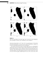
removing “salt and pepper” noise while preserving the fine image details. Figures 12.7(a)
and (b) depict a noise free grayscale image and the corresponding image with “salt and
pepper”noise. Each pixel in the image has a 10 percent probability of being contaminated
with an impulse. The impulses occur randomly and were generated by M
ATLAB’s imnoise
funtion. Figures 12.7(c) and (d) depict the noisy image processed with a 5 ϫ 5 window
CWM smoother with center weights 15 and 5, respectively. The impulse-rejection and
detail-preservation tradeoff in CWM smoothing is clearly illustrated in Figs. 12.7(c) and
12.7(d). A color version of the “port rait” image was also corrupted by “salt and pepper”
noise and filtered using CWM independently in each color plane.
At the extreme, for W
c
ϭ 1, the CWM smoother reduces to the median smoother
which is effective at removing impulsive noise. It is, however, unable to preserve the
image’s fine details [22]. Figure 12.9 shows enlarged sections of the noise-free image
278 CHAPTER 12 Nonlinear Filtering for Image Analysis and Enhancement

(a) (b)
(c) (d)
FIGURE 12.7
Impulse noise cleaning with a 5 ϫ 5 CWM smoother: (a) original grayscale “portrait” image;
(b) image with salt and pepper noise; (c) CWM smoother with W
c
ϭ 15; (d) CWM smoother with
W
c
ϭ 5.
12.3 Image Noise Cleaning 279
(a) (b)
(c)
(d)
FIGURE 12.8
Impulse noise cleaning with a 5 ϫ 5 CWM smoother: (a) original “portrait” image; (b) image with
salt and pepper noise; (c) CWM smoother with W
c
ϭ 16; (d) CWM smoother with W
c
ϭ 5.
280 CHAPTER 12 Nonlinear Filtering for Image Analysis and Enhancement
FIGURE 12.9
(Enlarged) Noise-free image (left); 5 ϫ 5 median smoother output (center); and 5 ϫ 5 mean
smoother (right).
(left), and of the noisy image after the median smoother has been applied (center). Severe
blurring is introduced by the median smoother and it is readily apparent in Fig. 12.9.
As a reference, the output of a running mean of the same size is also shown in Fig. 12.9
(right). The image is severely degraded as each impulse is smeared to neighboring pixels
by the averaging operation.

Figures 12.7 and 12.8 show that CWM smoothers can be effective at removing impul-
sive noise. If increased detail-preservation is sought and the center weight is increased,
CWM smoothers begin to breakdown and impulses appear on the output. One simple
way to ameliorate this limitation is to employ a recursive mode of operation. In essence,
past inputs are replaced by previous outputs as described in (12.12) with the only dif-
ference that only the center sample is weighted. All the other samples in the window are
weighted by one. Figure 12.10 shows enlarged sections of the nonrecursive CWM filter
(left) and of the corresponding recursive CWM smoother, both with the same center
weight (W
c
ϭ 15). This figure illustrates the increased noise attenuation provided by
recursion without the loss of image resolution.
Both recursive and nonrecursive CWM smoothers can produce outputs with dis-
turbing artifacts particularly when the center weights are increased in order to improve
12.3 Image Noise Cleaning 281
FIGURE 12.10
(Enlarged) CWM smoother output (left); recursive CWM smoother output (center); and permu-
tation CWM smoother output (right). Window size is 5 ϫ 5.
the detail-preservation characteristics of the smoothers. The artifacts are most apparent
around the image’s edges and details. Edges at the output appear jagged and impulsive
noise can break through next to the image detail features. The distinct response of the
CWM smoother in different regions of the image is due to the fact that images are non-
stationary in nature. Abrupt changes in the image’s local mean and texture carr y most
of the visual information content. CWM smoothers process the entire image with fixed
weights and are inherently limited in this sense by their static nature. Although some
improvement is attained by introducing recursion or by using more weights in a properly
designed WM smoother structure, these approaches are also static and do not properly
address the nonstationary nature of images.
Significant improvement in noise attenuation and detail preservation can be attained
if permutation WM filter structures are used. Figure 12.10 (right) shows the output of the

permutation CWM filter in (12.15) when the “salt and pepper”degraded“portrait”image
is inputted. The parameters were given the values T
L
ϭ 6 and T
U
ϭ 20. The improvement
achieved by switching W
c
between just two different values is significant. The impulses
are deleted without exception, the details are preserved, and the jagged artifacts typical
of CWM smoothers are not present in the output.
282 CHAPTER 12 Nonlinear Filtering for Image Analysis and Enhancement
12.4 IMAGE ZOOMING
Zooming an image is an important task used in many applications, including the World
Wide Web,digital video,DVDs,and scientific imaging. When zooming, pixels are inserted
into the image in order to expand the size of the image, and the major task is the inter-
polation of the new pixels from the surrounding original pixels. Weighted medians have
been applied to similar problems requiring interpolation, such as interlace to progressive
video conversion for television systems [13]. The advantage of using the WM in interpo-
lation over traditional linear methods is better edge preservation and a less “blocky” look
to edges.
To introduce the idea of interpolation, suppose that a small matrix must be zoomed
by a factor of 2, and the median of the closest two (or four) original pixels is used to
interpolate each new pixel:

785
6109

Zero
Interlace

ϪϪϪϪϪ→
⎡
⎢
⎢
⎢
⎣
70 8 050
00 0 000
6010090
00 0 000
⎤
⎥
⎥
⎥
⎦
Median
Interpolation
ϪϪϪϪϪϪϪ→
⎡
⎢
⎢
⎢
⎣
7 7.5 8 6.5 5 5
6.5 7.5 9 8.5 7 7
6 8 10 9.5 9 9
6 8 10 9.5 9 9
⎤
⎥
⎥

⎥
⎦
.
Zooming commonly requires a change in the image dimensions by a noninteger
factor, such as a 50% zoom where the dimensions must be 1.5 times the original. Also, a
change in the length-to-width ratio might be needed if the horizontal and vertical zoom
factors are different. The simplest way to accomplish zooming of arbitrary scale is to
double the size of the original as many times as needed to obtain an image larger than
the target size in all dimensions, interpolating new pixels on each expansion. Then the
desired image can be attained by subsampling the larger image, or taking pixels at regular
intervals from the larger image in order to obtain an image with the correct length and
width. The subsampling of images and the possible filtering needed are topics well known
in traditional image processing, thus, we will focus on the problem of doubling the size
of an image.
A digital image is represented by an array of values, each value defining the color of a
pixel of the image. Whether the color is constrained to be a shade of gray, i n which case
only one value is needed to define the brightness of each pixel, or whether three values
are needed to define the red, green, and blue components of each pixel does not affect the
definition of the technique of WM interpolation. The only difference between grayscale
and color images is that an ordinar y WM is used in grayscale images while color requires
a vector WM.
12.4 Image Zooming 283
To double the size of an image, first an empt y array is constructed with twice the
number of rows and columns as the original (Fig. 12.11(a)), and the original pixels are
placed into alternating rows and columns (the“00”pixels in Fig. 12.11(a)). To interpolate
the remaining pixels, the method known as polyphase interpolation is used. In this
method, each new pixel with four original pixels at its four corners (the “11” pixels in
Fig. 12.11(b)) is interpolated first by using the WM of the four nearest original pixels
as the value for that pixel. Since all original pixels are equally trustworthy and the same
distance from the pixel being interpolated, a weight of 1 is used for the four nearest

original pixels. The resulting array is shown in Fig. 12.11(c). The remaining pixels are
determined by taking a WM of the four closest pixels. Thus each of the “01” pixels
in Fig. 12.11(c) is interpolated using two original pixels to the left and right and two
previously interpolated pixels above and below. Similarly, the “10” pixels are interpolated
with original pixels above and below and interpolated pixels (“11” pixels) to the right
and left.
Since the “11” pixels were interpolated, they are less reliable than the original pixels
and should be given lower weights in determining the“01”and“10” pixels. Therefore, the
“11” pixels are given weights of 0.5 in the median to determine the “01” and “10” pixels,
while the “00” original pixels have weights of 1 associated with them. The weight of 0.5
is used because it implies that when both “11” pixels have values that are not between
the two “00” pixel values then one of the “00” pixels or their average will be used. Thus
“11” pixels differing from the “00”pixels do not greatly affect the result of the WM. Only
when the “11” pixels lie between the two “00” pixels will they have a direct effect on the
interpolation. The choice of 0.5 for the weight is arbitrary, since any weight greater than 0
and less than 1 will produce the same result. When implementing the polyphase method,
the “01” and “10” pixels must be treated differently due to the fact that the orientation
of the two closest original pixels is different for the two types of pixels. Figure 12.11(d)
shows the final result of doubling the size of the original array.
To illustrate the process, consider an expansion of the grayscale image represented by
an array of pixels, the pixel in the ith row and jth column having brightness a
i,j
. The array
a
i,j
will be interpolated into the array x
pq
i,j
, with p and q taking values 0 or 1 indicating in
the same way as above the type of interpolation required:

⎡
⎣
a
1,1
a
1,2
a
1,3
a
2,1
a
2,2
a
2,3
a
3,1
a
3,2
a
3,3
⎤
⎦
”
⎡
⎢
⎢
⎢
⎢
⎢
⎢

⎢
⎢
⎢
⎢
⎢
⎢
⎢
⎣
x
00
1,1
x
01
1,1
x
00
1,2
x
01
1,2
x
00
1,3
x
01
1,3
x
10
1,1
x

11
1,1
x
10
1,2
x
11
1,2
x
10
1,3
x
11
1,3
x
00
2,1
x
01
2,1
x
00
2,2
x
01
2,2
x
00
2,3
x

01
2,3
x
10
2,1
x
11
2,1
x
10
2,2
x
11
2,2
x
10
2,3
x
11
2,3
x
00
3,1
x
01
3,1
x
00
3,2
x

01
3,2
x
00
3,3
x
01
3,3
x
10
3,1
x
11
3,1
x
10
3,2
x
11
3,2
x
10
3,3
x
11
3,3
⎤
⎥
⎥
⎥

⎥
⎥
⎥
⎥
⎥
⎥
⎥
⎥
⎥
⎥
⎦
.
284 CHAPTER 12 Nonlinear Filtering for Image Analysis and Enhancement
00 01 00 01 00 01
10 11 10 11 10 11
00 01 00 01 00 01
10 11 10 11 10 11
00 01 00 01 00 01
10 11 10 11 10 11
01
01
01
10 11 10 11 10 11
01 01 01
10 11 10 11 10 11
01 01 01
10 11 10 11 10 11
(a) (b)
01 01 01
10 10 10

01 01 01
10 10 10
01 01 01
10 10 10
(c) (d)
FIGURE 12.11
The steps of polyphase interpolation.
The pixels are interpolated as follows:
x
00
i,j
ϭ a
i,j
x
11
i,j
ϭ MEDIAN[a
i,j
, a
iϩ1,j
, a
i,jϩ1
, a
iϩ1,jϩ1
]
x
01
i,j
ϭ MEDIAN[a
i,j

, a
i,jϩ1
, 0.5 x
11
iϪ1,j
, 0.5 x
11
iϩ1,j
]
x
10
i,j
ϭ MEDIAN[a
i,j
, a
iϩ1,j
, 0.5 x
11
i,jϪ1
, 0.5 x
11
i,jϩ1
].
An example of median interpolation compared with bilinear interpolation is given
in Fig. 12.12. Bilinear interpolation uses the average of the nearest two original pixels to
interpolate the “01” and “10” pixels in Fig. 12.11(b) and the average of the nearest four
original pixels forthe“11”pixels. The edge-preserving advantage of theWM interpolation
is readily seen in the figure.
12.5 IMAGE SHARPENING
Human perception is highly sensitive to edges and fine details of an image and since they

are composed primarily high-frequency components, the visual quality of an image can
be enormously degraded if the high frequencies are attenuated or completely removed.
12.5 Image Sharpening 285
FIGURE 12.12
Example of zooming. Original is at the top with the area of interest outlined in white. On the
lower left is the bilinear interpolation of the area, and on the lower right the weighted median
interpolation.
On the other hand, enhancing the high-frequency components of an image leads to an
improvement in the visual quality. Image sharpening refers to any enhancement technique
that hig hlights edges and fine details in an image. Image sharpening is widely used in
printing and photographic industries for increasing the local contrast and sharpening the
images. In principle, image sharpening consists of adding to the or iginal image a signal
that is proportional to a highpass filtered version of the original image. Figure 12.13
illustrates this procedure often referred to as unsharp masking [23, 24] on a 1D signal. As
shown in Fig. 12.13, the original image is first filtered by a highpass filter which extracts
the high-frequency components, and then a scaled version of the highpass filter output
286 CHAPTER 12 Nonlinear Filtering for Image Analysis and Enhancement
Highpass
filter
3
1
Original
signal
1
1
l
Sharpened
signal
FIGURE 12.13
Image sharpening by high-frequency emphasis.

is added to the original image thus producing a sharpened image of the original. Note
that the homogeneous regions of the signal, i.e., where the signal is constant, remain
unchanged. The sharpening operation can be represented by
s
i,j
ϭ x
i,j
ϩ ␭ ∗F(x
i,j
), (12.28)
where x
i,j
is the original pixel value at the coordinate (i,j), F(·) is the highpass filter,
␭ is a tuning parameter greater than or equal to zero, and s
i,j
is the sharpened pixel at
the coordinate (i,j). The value taken by ␭ depends on the grade of sharpness desired.
Increasing ␭ yields a more sharpened image.
If color images are used, x
i,j
, s
i,j
, and ␭ are three-component vectors, whereas if
grayscale images are used, x
i,j
, s
i,j
, and ␭ are single-component vectors. Thus the process
described here can be applied to either grayscale or color images with the only difference
that vector-filters have to be used in sharpening color images whereas single-component

filters are used with grayscale images.
The key point in the effective sharpening process lies in the choice of the highpass
filtering operation. Traditionally, linear filters have been used to implement the highpass
filter, however, linear techniques can lead to unacceptable results if the original image is
corrupted with noise. A trade-off between noise attenuation and edge highlighting can
be obtained if a WM filter with appropriated weights is used. To illustrate this, consider
a WM filter applied to a grayscale image where the following filter mask is used
W ϭ
1
3
⎡
⎢
⎣
Ϫ1 Ϫ1 Ϫ1
Ϫ18Ϫ1
Ϫ1 Ϫ1 Ϫ1
⎤
⎥
⎦
. (12.29)
Due to the weight coefficients in (12.29), for each position of the moving window, the
output is proportional to the difference between the center pixel and the smallest pixel
around the center pixel. Thus, the filter output takes relatively large values for prominent
12.5 Image Sharpening 287
edges in an image, and small values in regions that are fairly smooth, being zero only in
regions that have constant gray level.
Although this filter can effectively extract the edges contained in a image, the effect
that this filtering operation has over negative-slope edges is different from that obtained
for positive-slope edges.
1

Since the filter output is proportional to the difference between
the center pixel and the smallest pixel around the center, for negative-slope edges, the
center pixel takes small values producing small values at the filter output. Moreover, the
filter output is zero if the smallest pixel around the center pixel and the center pixel
have the same values. This implies that negative-slope edges are not extracted in the
same way as positive-slope edges. To overcome this limitation, the basic image sharpen-
ing structure shown in Fig. 12.13 must be modified such that positive-slope edges and
negative-slope edges are highlighted in the same proportion. A simple way to accomplish
that is: (a) extract the positive-slope edges by filtering the original image with the filter
mask descr ibed above; (b) extract the negative-slope edges by first preprocessing the
original image such that the negative-slope edges become positive-slope edges, and then
filter the preprocessed image with the filter described above; and (c) combine appropri-
ately the original image, the filtered version of the original image and the filtered version
of the preprocessed image to form the sharpened image.
Thus both positive-slope edges and negative-slope edges are equally highlighted. This
procedureisillustratedinFig. 12.14, where the top br anch extracts the positive-slope
edges and the middle branch extracts the negative-slope edges. In order to understand
the effects of edge sharpening , a row of a test image is plotted in Fig. 12.15 together
with a row of the sharpened image when only the positive-slope edges are highlighted
(Fig. 12.15(a)), only the negative-slope edges are highlighted (Fig. 12.15(b)), and both
positive-slope and negative-slope edges are jointly highlighted (Fig. 12.15(c)).
In Fig. 12.14, ␭
1
and ␭
2
are tuning parameters that control the amount of sharpness
desired in the positive-slope direction and in the negative-slope direction, respectively.
The values of ␭
1
and ␭

2
are generally selected to be equal. The output of the pre-filtering
operation is defined as
x
Ј
i,j
ϭ M Ϫ x
i,j
(12.30)
with M equal to the maximum pixel value of the original image. This pre-filtering
operation can be thought of as a flipping and a shifting operation of the values of the
original image such that the negative-slope edges are converted to positive-slope edges.
Since the original image and the pre-filtered image are filtered by the same WM filter, the
positive-slope edges and negative-slope edges are sharpened in the same way.
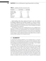
In Fig. 12.16, the performance of the WM filter image sharpening is compared with
that of traditional image sharpening based on linear FIR filters. For the linear sharpener,
the scheme shown in Fig. 12.13 was used. The parameter ␭ was set to 1 for the clean
1
A change from a gray level to a lower gr ay level is referred to as a negative-slope edge, whereas a change
from a gray level to a higher gray level is referred to as a positive-slope edge.
288 CHAPTER 12 Nonlinear Filtering for Image Analysis and Enhancement
Highpass
WM filter
Highpass
WM filter
Pre-filtering
1
1
1
1

1
2
3
l
2
l
1
3
FIGURE 12.14
Image sharpening based on the weighted median filter.
(a) (b) (c)
FIGURE 12.15
Original row of a test image (solid line) and row sharpened (dotted line) with (a) only positive-slope
edges; (b) only negative-slope edges; and (c) both positive-slope and negative-slope edges.
image and to 0.75 for the noise image. For the WM sharpener, the scheme of Fig. 12.14
was used with ␭
1
ϭ ␭
2
ϭ 2 for the clean image, and ␭
1
ϭ ␭
2
ϭ 1.5 for the noisy image.
The filter mask given by (12.29) was used in both linear and median image sharpening.
As before each component of the color image was processed separately.
12.6 Conclusion 289
(a) (b) (c)
(d) (e) (f)
FIGURE 12.16

(a) Original image sharpened with; (b) the FIR-sharpener; and (c) the WM-sharpener;
(d) Image with added Gaussian noise sharpened with; (e) the FIR-sharpener; and (f) the
WM-sharpener.
12.6 CONCLUSION
The principles behind WM smoothers and WM filters have been presented in this
chapter, as well as some of the applications of these nonlinear signal processing str uc-
tures in image enhancement. It should be apparent to the reader that many similarities
exist between linear and median filters. As illustrated in this chapter, there are several
applications in image enhancement where WM filters provide significant advantages
over traditional image enhancement methods using linear filters. The methods pre-
sented here, and other image enhancement methods that can be easily developed
using WM filters, are computationally simple and provide significant advantages, and
consequently can be used in emerging consumer electronic products, PC and internet
imaging tools, medical and biomedical imaging systems, and of course in militar y
applications.
290 CHAPTER 12 Nonlinear Filtering for Image Analysis and Enhancement
ACKNOWLEDGMENT
This work was supported in part by the NATIONAL SCIENCE FOUNDATION under grant
MIP-9530923.
REFERENCES
[1] Y. H. Lee and S. A. Kassam. Generalized median filtering and related nonlinear filtering techniques.
IEEE Trans. Acoust., 33:672–683, 1985.
[2] J. W. Tukey. Nonlinear (nonsuperimposable) methods for smoothing data. In Conf. Rec., (Eascon),
1974.
[3] T. A. Nodes and N. C. Gallagher, Jr. Median filters: some modifications and their properties. IEEE
Trans. Acoust., 30:739–746, 1982.
[4] G. R. Arce and N. C. Gallagher, Jr. Stochastic analysis of the recursive median filter process. IEEE
Trans. Inf. Theory, IT-34:669–679, 1988.
[5] G. R. Arce. Statistical threshold decomposition for recursive and nonrecursive median filters. IEEE
Trans. Inf. Theory, 32:243–253, 1986.

[6] E. L. Lehmann. Theory of Point Estimation. J Wiley & Sons, New York, NY, 1983.
[7] A. C. Bovik, T. S. Huang, and J. D.C. Munson. A generalization of median filtering using linear
combinations of order statistics. IEEE Trans. Acoust., 31:1342–1350, 1983.
[8] H. A. David. Order Statistics. Wiley Interscience, New York, 1981.
[9] B. C. Arnold, N. Balakrishnan, and H. N. Nagaraja. A First Course in Order Statistics. John Wiley &
Sons, New York, NY, 1992.
[10] F. Y. Edgeworth. A new method of reducing observations relating to several quantities. Phil. Mag.
(Fifth Series), 24:222–223, 1887.
[11] D. R. K. Brownrigg. The weighted median filter. Commun. ACM, 27:807–818, 1984.
[12] S J. Ko and Y. H. Lee. Center weighted median filters and their applications to image enhancement.
Theor. Comput. Sci., 38:984–993, 1991.
[13] L. Yin, R. Yang, M. Gabbouj, and Y. Neuvo. Weighted median filters: a tutorial. IEEE Trans. Circuits
Syst. II, 41:157–192, 1996.
[14] O. Yli-Harja, J. Astola, and Y. Neuvo. Analysis of the properties of median and weighted median
filters using threshold logic and stack filter representation. IEEE Trans. Acoust., 39:395–410, 1991.
[15] G. R. Arce, T. A. Hall, and K. E. Barner. Permutation weighted order statistic filters. IEEE Trans.
Image Process., 4:1070–1083, 1995.
[16] R. C. Hardie and K. E. Barner. Rank conditioned rank selection filters for signal restoration. IEEE
Trans Image Process., 3:192–206, 1994.
[17] J. P. Fitch, E. J. Coyle, and N. C. Gallagher. Median filtering by threshold decomposition. IEEE
Trans. Acoust., 32:1183–1188, 1984.
[18] P. D. Wendt, E. J. Coyle, and N. C. Gallagher, Jr. Stack filters. IEEE Trans. Acoust., 34:898–911, 1986.
[19] E. N. Gilbert. Lattice-theoretic properties of frontal switching functions. J. Math. Phys., 33:57–67,
1954.
References 291
[20] G. R. Arce. A general weighted median filter structure admitting negative weights. IEEE Trans.
Signal Process., 46:3195–3205, 1998.
[21] J. L. Paredes and G. R. Arce. Stack filters, stack smoothers, and mirrored threshold decomposition.
IEEE Trans. Signal Process., 47:2757–2767, 1999.
[22] A. C. Bovik. Streaking in median filtered images. IEEE Trans. Acoust., 35:493–503, 1987.

[23] A. K. Jain. Fundamentals of Digital Image Processing. Prentice Hall, Upper Saddle River, New Jersey,
1989.
[24] J. S. Lim. Two-Dimensional Signal and Image Processing. Prentice Hall, Englewood Cliffs, NJ, 1990.
[25] S. Hoyos,Y. Li, J. Bacca, and G. R. Arce. Weighted median filters admitting complex-valued weights
and their optimization. IEEE Trans. Acoust., 52:2776–2787, 2004.
[26] S. Hoyos, J. Bacca, and G. R. Arce. Spectral design of weighted median filters: a general iterative
approach. IEEE Trans. Acoust., 53:1045–1056, 2005.
CHAPTER
13
Morphological Filtering
Petros Maragos
National Technical University of Athens
13.1 INTRODUCTION
The goals of image enhancement include the improvement of the visibility and per-
ceptibility of the various regions into which an image can be partitioned and of the
detectability of the image features inside these regions. These goals include tasks such
as cleaning the image from various types of noise, enhancing the contrast among adja-
cent regions or features, simplifying the image via selective smoothing or elimination of
features at certain scales, and retaining only features at certain desirable scales. Image
enhancement is usually followed by (or is done simultaneously with) detect ion of features
such as edges, peaks, and other geometric features, which is of paramount importance in
low-level vision. Further, many related vision problems involve the detection of a known
template; such problems are usually solved via template matching.
While traditional approaches for solving the above tasks have used mainly tools of
linear systems, nowadays a new understanding has matured that linear approaches are not
well suited or even fail to solve problems involving geometrical aspects of the image. Thus,
there is a need for nonlinear geometric approaches. A powerful nonlinear methodology
that can successfully solve the above problems is mathematical morphology.
Mathematical morphology is a set- and lattice-theoretic methodology for image ana-
lysis, which aims at quantitatively describing the geometrical structure of image objects.

It was initiated [1, 2] in the late 1960s to analyze binary images from geolog ical and
biomedical data as well as to formalize and extend earlier or parallel work [3, 4] on
binary pattern recognition based on cellular automata and Boolean/threshold logic. In
the late 1970s, it was extended to gray-level images [2]. In the mid-1980s, it was brought
to the mainstream of image/signal processing and related to other nonlinear filtering
approaches [5, 6]. Finally, in the late 1980s and 1990s, it was generalized to arbitrary
lattices [7, 8]. The above evolution of ideas has formed what we call nowadays the field
of morphological image processing, which is a broad and coherent collection of theore-
tical concepts, nonlinear filters, design methodologies, and applications systems. Its rich
theoretical framework, algorithmic efficiency, easy implementability on special hardware,
and suitability for many shape-oriented problems have propelled its widespread usage
293
294 CHAPTER 13 Morphological Filtering
and further advancement by many academic and industry groups working on various
problems in image processing, computer vision, and pattern recognition.
This chapter provides a brief introduction to the application of morphological image
processing to image enhancement and feature detection. Thus, it discusses four important
general problems of low-level (early) vision, progressing from the easiest (or more easily
defined) to the more difficult (or harder to define): (i) geometric filtering of binary
and gray-level images of the shrink/expand type or of the peak/valley blob removal type;
(ii) cleaning noise fromthe image or improving its contrast; (iii) detecting in the image the
presence of known templates; and (iv) detecting the existence and location of geometric
features such as edges and peaks whose types are known but not their exact form.
13.2 MORPHOLOGICAL IMAGE OPERATORS
13.2.1 Morphological Filters for Binary Images
Given a sampled
1
binary image signal f [x] with values 1 for the image object and 0 for
the background, typical image transformations involving a moving window set W ϭ
{y

1
,y
2
, , y
n
} of n sample indexes would be
␺
b
( f )[x] ϭ b( f [x Ϫ y
1
], , f [x Ϫ y
n
]), (13.1)
where b(v
1
, , v
n
) is a Boolean function of n variables. The mapping f → ␺
b
( f ) is
called a Boolean filter. By varying the Boolean function b, a large variety of Boolean
filters can be obtained. For example, choosing a Boolean AND for b would shrink the
input image object, whereas a Boolean OR would expand it. Numerous other Boolean
filters are possible since there are 2
2
n
possible Boolean functions of n variables. The main
applications of such Booleanimage operations have been in biomedical image processing,
character recognition, object detection, and gener al 2D shape analysis [3, 4].
Among the important concepts offered by mathematical morphology was to use sets

to represent binary images and set operations to represent binary image transformations.
Specifically, given a binary image, let the object be represented by the set X and its
background by the set complement X
c
. The Boolean OR transformation of X by a
(window) set B is equivalent to the Minkowski set a ddition ⊕, also called dilation,ofX
by B:
X ⊕B  {z : (B
s
)
ϩz
∩X ϭл}ϭ

y∈B
X
ϩy
, (13.2)
where X
ϩy
 {x ϩ y : x ∈ X} is the translation of X along the vector y, and B
s
 {x :
Ϫx ∈ B} is the symmetr ic of B with respect to the origin. Likewise, the Boolean AND
1
Signals of a continuous variable x ∈ R
m
are usually denoted by f (x), whereas for signals with discrete
variable x ∈
Z
m

we write f [x]. R and Z denote, respectively, the set of reals and integers.
13.2 Morphological Image Operators 295
transformation of X by B
s
is equivalent to the Minkowski set subtraction , also called
erosion,ofX by B:
X B  {z : B
ϩz
⊆ X} ϭ

y∈B
X
Ϫy
. (13.3)
Cascading erosion and dilation creates two other operations, the Minkowski opening
X
◦B  (X B) ⊕B and the closing X •B  (X ⊕B) B of X by B. In applications,
B is usually called a structuring eleme nt and has a simple geometrical shape and a size
smaller than the image X.IfB has a regular shape, e.g ., a small disk, then both opening
and closing act as nonlinear filters that smooth the contours of the input image. Namely,
if X is viewed as a flat island, the opening suppresses the sharp capes and cuts the narrow
isthmuses of X, whereas the closing fills in the thin gulfs and small holes.
Thereisaduality between dilation and erosion since X ⊕B ϭ (X
c
B
s
)
c
; i.e.,
dilation of an image object by B is equivalent to eroding its background by B

s
and
complementing the result. A similar duality exists between closing and opening.
13.2.2 Morphological Filters for Gray-level Images
Extending morphological operators from binary to gray-level images can be done by
using set representations of signals and transforming these input sets via morphological
set operations. Thus, consider an image signal f (x) defined on the continuous or discrete
plane E ϭ R
2
or Z
2
and assuming values in R ϭ R ∪{Ϫϱ,ϱ}. Thresholding f at all
amplitude levels v produces an ensemble of binary images represented by the upper level
sets (also called threshold sets):
X
v
( f )  {x ∈E : f (x) Ն v}, Ϫϱ < v < ϩϱ. (13.4)
The image can be exactly reconstructed from all its level sets since
f (x) ϭ sup{v ∈R : x ∈ X
v
( f )}, (13.5)
where “sup” denotes supremum.
2
Transforming each level s et of the input signal f by a
set operator ⌿ and viewing the transformed sets as level sets of a new image creates [2, 5]
a flat image operator ␺, whose output signal is
␺( f )(x) ϭ sup{v ∈R : x ∈ ⌿[X
v
( f )]}. (13.6)
2

GivenasetX of real numbers, the supremum of X is its lowest upper bound. If X is finite (or infinite but
closed from above), its supremum coincides with its maximum.
296 CHAPTER 13 Morphological Filtering
For example, if ⌿ is the set dilation and erosion by B, the above procedure creates the
two most elementary morphological image operators: the dilation and erosion of f (x)
byasetB:
( f ⊕B)(x) 

y∈B
f (x Ϫ y), (13.7)
( f B)(x) 

y∈B
f (x ϩ y), (13.8)
where

denotes supremum (or maximum for finite B) and

denotes infimum (or
minimum for finite B). Flat erosion (dilation) of a function f by a small convex set B
reduces (increases) the peaks (valleys) and enlarges theminima (maxima) of the function.
The flat opening f
◦B ϭ ( f B) ⊕B of f by B smooths the graph of f from below by
cutting down its peaks, whereas the closing f
•B ϭ ( f ⊕B) B smooths it from above
by filling up its valleys.
The most general translation-invariant morphological dilation and erosion of a gray-
level image signal f (x) by another signal g are:
( f ⊕g)(x) 


y∈E
f (x Ϫ y) ϩ g(y), (13.9)
( f g)(x) 

y∈E
f (x ϩ y) Ϫ g(y). (13.10)
Note that signal dilation is a nonlinear convolution where the sum-of-products in the
standard linear convolution is replaced by a max-of-sums.
13.2.3 Universality of Morphological Operators
3
Dilations or erosions can be combined in many ways to create more complex morpholo-
gical operators that can solve a broad variety of problems in image analysis and nonlinear
filtering. Their versatility is further strengthened by a theory outlined in [5, 6] that
represents a broad class of nonlinear and linear operators as a minimal combination of
erosions or dilations. Here we summarize the main results of this theory restricting our
discussion only to discrete 2D image signals.
Any translation-invariant set operator ⌿ is uniquely characterized by its kernel
Ker(⌿)  {X ∈ Z
2
:0∈ ⌿(X)}.If ⌿ is also increasing (i.e., X ⊆ Y ” ⌿(X) ⊆ ⌿(Y )),
then it can be represented as a union of erosions by all its kernel sets [1]. However, this
kernel representation requires an infinite number of erosions. A more efficient (requir-
ing less erosions) representation uses only a substructure of the kernel, its basis Bas(⌿),
defined as the collection of kernel elements that are minimal with respect to the par-
tial ordering ⊆.If⌿ is also upper se micontinuous (i.e., ⌿(

n
X
n
) ϭ


n
⌿(X
n
) for any
3
This is a section for mathematically-inclined readers and can be skipped without significant loss of
continuity.
13.2 Morphological Image Operators 297
decreasing set sequence (X
n
)), then ⌿ has a nonempty basis and can be represented
exactly as a union of erosions by its basis sets:
⌿(X) ϭ

A∈Bas(⌿)
X A. (13.11)
The morphological basis representation has also been extended to gray-level signal
operators. As a special case, if ␾ is a flat signal operator as in (13.6) that is translation-
invariant and commutes with thresholding, then ␾ can be represented as a supremum of
erosions by the basis sets of its corresponding set operator ⌽:
␾( f ) ϭ

A∈Bas(⌽)
f A. (13.12)
By duality, there is also an alternative representation where a set operator ⌿ satisfying
the above three assumptions can be realized exactly as the intersection of dilations by the
reflected basis sets of its dual operator ⌿
d
(X)  [⌿(X

c
)]
c
. There is also a similar dual
representation of signal operators as an infimum of dilations.
Given the wide applicability of erosions/dilations, their parallellism, and their simple
implementations, the morphological representation theory supports a general purpose
image processing (software or hardware) module that can perform erosions/dilations,
based on which numerous other complex image operations can be built.
13.2.4 Median, Rank, and Stack Filters
Flat erosion and dilation of a discrete image signal f [x] by a finite window W ϭ
{y
1
, , y
n
}⊆Z
2
is a moving local minimum or maximum. Replacing min/max with
a more general rank leads to rank filters. At each location x ∈ Z
2
, sorting the signal values
within the reflected and shifted n-point window (W
s
)
ϩx
in decreasing order and picking
the p-th largest value, p ϭ 1,2, ,n, yields the output signal from the pth rank filter:
( f ✷
p
W )[x]  pth rank of (f [x Ϫ y

1
], , f [x Ϫ y
n
]). (13.13)
For odd n and p ϭ (n ϩ 1)/2 we obtain the median filter. Rank filters and especially
medians have been applied mainly to suppress impulse noise or noise whose probability
density has heavier tails than the Gaussian for enhancement of image and other signals,
since they can remove this type of noise without blurring edges, as would be the case for
linear filtering.
If the input image is binary, the rank filter output is also binary since sorting preserves
a signal’s range. Rank filtering of binary images involves only counting of points and no
sorting. Namely, if the set S ⊆ Z
2
represents an input binary image, the output set
produced by the pth rank set filter is
S✷
p
W  {x : card[(W
s
)
ϩx
∩S]Ն p}, (13.14)
where card(X) denotes the cardinality (i.e., number of points) of a set X.
All rank operators commute with thresholding; i.e.,
X
v
[f ✷
p
W ] ϭ [X
v

( f )]✷
p
W , ∀v, ∀p (13.15)
298 CHAPTER 13 Morphological Filtering
where X
v
( f ) is the level set (binary image) resulting from thresholding f at level v.
This property is also shared by all morphological operators that are finite compositions
or maxima/minima of flat dilations and erosions by finite structuring elements. All
such signal operators ␺ that have a corresponding set operator ⌿ and commute with
thresholding can be alternatively implemented via threshold superp osition as in (13.6).
Further, since the binary version of all the above discrete translation-invariant finite-
window operators can be described by their generating Boolean function as in (13.1),all
that is needed in synthesizing their corresponding gray-level image filters is knowledge
of this Boolean function. Specifically, let f
v
[x] be the binary images represented by the
threshold sets X
v
( f ) of an input gray-level image f [x]. Transforming all f
v
with an
increasing (i.e., containing no complemented variables) Boolean function b(u
1
, , u
n
)
in place of the set operator ⌿ in (13.6) and using threshold superposition creates a class
of nonlinear digital filters called stack filters [5, 9]:
␾

b
( f )[x]  sup{v ∈ R : b( f
v
[x Ϫ y
1
], , f
v
[x Ϫ y
n
]) ϭ 1}. (13.16)
The use of Boolean functions facilitates the design of such discrete flat operators
with determinable st ructural properties. Since each increasing Boolean function can be
uniquely represented by an irreducible sum (product) of product (sum) terms, and each
product (sum) term corresponds to an erosion (dilation), each stack filter can be repre-
sented as a finite maximum (minimum) of flat erosions (dilations) [5]. For example, the
window W ϭ {Ϫ1,0,1} and the Boolean function b
1
(u
1
,u
2
,u
3
) ϭ u
1
u
2
ϩ u
2
u

3
ϩ u
1
u
3
create a stack filter that is identical to the 3-point median by W, which can also be
represented as a maximum of three 2-point erosions:
␾
b
( f )[x] ϭ median(f [x Ϫ 1],f [x],f [x ϩ 1])
(13.17)
ϭ max

min( f [x Ϫ 1],f [x]),min( f [x Ϫ 1],f [x ϩ 1]), min(f [x],f [x ϩ 1])

.
In general, because of their representation via erosions/dilations (which have a geometric
interpretation) and Boolean functions (which are related to mathematical logic), stack
filters can be analyzed or designed not only in terms of their statistical properties for
image denoising but also in terms of their geometric and logic properties for preserving
selected image str uctures.
13.2.5 Algebraic Generalizations of Morphological Operators
A more general formalization [7, 8] of morphological operators views them as operators
on complete lattices. A complete lattice isasetL equipped with a partial ordering Յ such
that (L,Յ) has the algebraic structure of a partially ordered se t where the supremum
and infimum of any of its subsets exist in L. For any subset K ⊆ L, its supremum

K and infimum

K are defined as the lowest (with respect to Յ) upper bound and

greatest lower bound of K, respectively. The two main examples of complete lattices used
in morphological image processing are (i) the space of all binary images represented
by subsets of the plane E where the

/

lattice operations are the setunion/intersection,