Part 2
Wind Turbine Controls

11
Control System Design
Yoonsu Nam
Department of Mechanical Engineering, Kangwon National University 192-1
Hyoja-2 dong, Chunchon, Kangwon 200-701
Korea
1. Introduction
A wind turbine control system is a complex and critical element in a wind turbine. It is
responsible for the autonomous, reliable, and safe operation of the machine in all wind
conditions. Two levels of control operations are required. One is supervisory control and the
other is dynamic feedback control of blade pitch and generator torque for maximizing
power production and minimizing mechanical loads on the wind turbine. The supervisory
control system is one operating system of the wind turbine and has the following functions:
• operational state (stand-by, start-up, power production, shutdown) transition control
• control of subsystems (cooling, heating, hydraulics, etc.)
• diagnostics, alarm management
• data logging, statistics, post-processing
• user access (management), visualization.
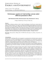
A supervisory controller monitors the turbine and wind condition in order to decide when
to start and shut down the wind turbine. Fig. 1 shows a schematic of the operational state
transition logic which is implemented in supervisory control. A wind turbine operator can
start and shut down turbine operation through a SCADA (supervisory control and data
acquisition) system as shown in Fig. 1. The SCADA system can communicate with the
supervisory controller in order to control and monitor the wind turbine.
The main topic of this chapter is the design of a control algorithm for the dynamic feedback
controller which manages the blade pitch, the generator torque, and the yaw system. Most
multi-MW wind turbines are equipped with variable speed and variable pitch (VSVP)
technology (Leithead

b
& Connor, 2000; Bianchi et al., 2007; Muller et al., 2002; Boukhezzar et
al., 2007). In the below rated wind speed conditions, the rotor speed varies with wind speed,
while the pitch is fixed in order to maximize the energy capture from the wind. However, in
the above rated wind speed conditions, the pitch is varied, while the rotor speed is fixed, in
order for the machine to produce the rated power. All the analysis and design issues
covered in this chapter for the dynamic feedback controller using VSVP technology target
an upwind type horizontal axis multi-MW wind turbine having 3 blades. Yawing control is
not dealt with here because of its simple on-off control logic. All the control algorithms
covered in this chapter are based on classical control theory (Franklin et al., 2006; Dorf &
Bishop, 2007).
This chapter is composed of 3 sections. Section 2 begins with a mathematical description of
the wind, which is not only the source of energy but also a disturbing input to the wind

Wind Turbines

268

Fig. 1. Schematic of a wind turbine control system
turbine. The wind turbine control strategy and structure based on VSVP technology are
explained. Simplified dynamic models of the pitch actuator and generator, which are
elements of the wind turbine control system, are followed. Section 3 covers dynamic
modeling and steady state characteristics of the wind turbine, based on a drive train model.
Variables comprising rotor speed, wind speed, and pitch angle completely specify an
operating condition of a wind turbine. How the dynamic characteristics vary with different
operating conditions is analyzed in this section. Finally, Section 4 presents the main topic of
this chapter, i.e. wind turbine control system design. It starts with the control system design
requirements which are determined from the wind characteristics and the aeroelastic
properties of the wind turbine structure. A methodology on how to set PI controller gains is
introduced, considering gain scheduling and the integrator anti-windup problem. The

section includes a feedforward pitch control system design using a wind speed estimator to
enhance the performance of the output power regulation. This section concludes with the
introduction of individual pitch control for mechanical load alleviation of the blades.
2. Wind turbine control system
2.1 Wind
Wind is highly variable. To accurately predict the wind ahead of time is almost impossible.
Statistical measures such as mean wind speed and turbulence intensity are frequently used.
Turbulence intensity is given by

I
v
σ
=
(1)
where σ is the standard deviation of the wind speed and
v is the mean wind speed, usually
defined for 10 minutes of wind data. Fig. 2 shows two different winds, even though these
have the same mean wind speed and turbulence intensity. One further statistical property,
Control System Design

269
i.e. autocorrelation, is necessary to discern the wind more specifically. The autocorrelation is
defined as

1
( ) { ( ) ( )} lim ( ) ( )
2
T
xx
T

T
Extxt xtxt dt
T
φτ τ τ
−
→∞
⎧
⎫
=+= +
⎨
⎬
⎩⎭
∫
(2)
where x(t) is a de-trended time series. Therefore, φ
xx
(0)=σ
x
2
. As signal frequency increases
and time-lag τ gets larger, the autocorrelation becomes smaller. The power spectral density,
which is the Fourier transform of the autocorrelation, is defined as

() ()
j
xx xx
ed
ωτ
ω
φτ τ

∞
−
−∞
Φ=
∫
. (3)
A sample of the autocorrelation and power spectral density for two different time series is
shown in Fig. 3.
Van der Hoven observed at Brookhaven, New York, in 1957 that there were distinct
periodicities in wind, as shown in Fig. 4 (van der Hoven, 1957). Three peaks, namely
synoptic, diurnal, and turbulent peaks, are clear in this plot. On a short time scale of less
than 2 hours, turbulent wind has most energy in the wind spectrum. The power spectral
density of turbulent wind can be modeled as

()
(
)
2
5/6
2
4/
()
1 70.8 /(2 )
uu
vv
u
Lv
Lv
σ
ω

ωπ
Φ=
+
(4)
where σ
u
is the standard deviation for a turbulent wind and L
u
is the length scale (Burton et
al., 2001). The length scale is a site-specific parameter and depends on the surface roughness
α and height
z . It is given by

0.35
280( / )
ui
Lzz= . (5)

0 0.2 0.4 0.6 0.8 1 1.2 1.4 1.6 1.8 2
5
10
15
time(sec)
v
2
(t)
0 0.2 0.4 0.6 0.8 1 1.2 1.4 1.6 1.8 2
5
10
15

time(sec)
v
1
(t)



Fig. 2. Two different winds with the same mean wind speed and turbulence intensity
Wind Turbines

270


Fig. 3. Autocorrelation and power spectral density
Some representative values of α are given in Table 1 with the value of z
i
. The turbulence
becomes isotropic for the condition of L
u
≥ 280 m at an altitude of z>z
i
. The above expression
of Eq. (4) is known as the von Karman spectrum in the longitudinal direction. The von
Karman expressions in the lateral and vertical directions can be found in the literature
(Burton et al., 2001).
2.2 Control system strategies and structure
The mechanical power of an air mass which has a flow rate of dm/dt with a constant speed of
v is given by

()

223
11 1
22 2
dd dm
PE mv v Av
dt dt dt
ρ
⎛⎞
== = =
⎜⎟
⎝⎠
(6)
where ρ is the air density and A is the cross sectional area of the air mass. Only a portion of
the wind power given by Eq. (6) is converted to electric power by a wind turbine. The
efficiency of the power conversion by a wind turbine depends on the aerodynamic design
and operational status of the wind turbine. Usually, the power generated by the wind
turbine is represented by

3
1
2
P
PC Av
ρ
⎛⎞
=
⎜⎟
⎝⎠
(7)
Control System Design


271


Fig. 4. van der Hoven wind spectrum

Type of terrain Roughness length α (m) z
i
=1000α
0.18
(m)
Cities, forests 0.7 937.8
Suburbs, wooded countryside 0.3 805.2
Villages, countryside with tress and hedges 0.1 660.7
Open farmland, few trees and buildings 0.03 532.0
Flat grassy plains 0.01 436.5
Flat desert, rough sea 0.001 288.4
Table 1. Surface roughness (Burton et al., 2001)
where Cp represents the efficiency of wind power conversion and is called the power
coefficient. The ideal maximum value of Cp is 16/27= 0.593, which is known as the Betz
limit (Manwell et al., 2009).
As shown in Fig. 5, the power coefficient, Cp is a function of pitch angle β and tip speed
ratio λ which is defined as

r
R
v
λ
Ω
=

(8)
where R is the rotor radius and Ω
r
is the rotor speed of the wind turbine. Fig. 5 is a sample
plot of Cp for a multi-MW wind turbine. The curve with dots shows the variation of Cp
with λ for a fixed pitch angle of β
0
. As the pitch angle is away from β
0
, the value of Cp
becomes smaller. Therefore, Cp has the maximum with the condition of λ=λ
0
and β =β
0
. In
order for a wind turbine to extract the maximum energy from the wind, the wind turbine
should be operated with the max-Cp condition. That is, the wind turbine should be
controlled to maintain the fixed tip speed ratio of λ =λ
0
with the fixed pitch of β =β
0
in spite of
varying wind speed. Referring to Eq. (8), there ought to be a proportional relationship between
the wind speed v and the rotor speed Ω
r
to keep the tip speed ratio at constant value of λ
0
.
Fig. 6 represents a power curve which consists of three operational regions. Region I is max-
Cp, Region II is a transition, and Region III is a power regulation region.

Wind Turbines

272



Fig. 5. Sample plot of Cp as a function of λ and β
•
Region I: The wind turbine is operated in max-Cp. The blade pitch angle is fixed at β
0

and the rotor speed is varied so as to maintain the tip speed ratio constant (λ
0
).
Therefore, the rotor speed is changed so as to be proportional to the wind speed by
controlling the generator reaction torque. In the max-Cp region, the generator torque
control is active only, while the blade pitch is fixed at β
0
.
•
Region II: This is a transition region between the other two regions, that is the max-Cp
(Region II) and power regulation region (Region III). Several requirements, such as a
smooth transition between the two regions, a blade-tip noise limit, minimal output
power fluctuations, etc., are important in defining control strategies for this region.
•
Region III: This is the above rated wind speed region, where wind turbine power is
regulated at the rated power. Therefore, rotor speed and generator reaction torque are
maintained at their rated values. In this region, the value of Cp has to be controlled so
as to be inversely proportional to v
3

to regulate the output power to the rated value.
This is easily found by noting Eq. (1). In this region, the blade pitch control plays a
major role in this task.
A control system structure for a wind turbine is shown schematically in Fig. 7. There are two
feedback loops. One is the pitch angle control loop and the other is the generator torque
control loop. Below the rated wind speed region, i.e. in Regions I and II, the blade pitch
angle is fixed at β
0
and the generator torque is controlled by a prescheduled look-up table
(see Section 3.2). The most common types of generator for a multi-MW wind turbine are a
doubly fed induction generator (DFIG) (Soter & Wegerer, 2007) and a permanent magnet

Control System Design

273


Fig. 6. Power curve
synchronous generator (PMSG) (Haque et al., 2010). These electric machines are complicated
mechanical and electric devices including AC-DC-AC power converters. For the purposes of
control system design, however, it is suffiicient to use a simple model of generator
dynamics:

2
22
()
() 2
gng
C
g

n
g
n
g
n
g
Ts
Ts s s
ω
ς
ωω
=
++
(9)
where T
g
C
is a generator torque command, ω
ng
(~ 40 r/s) is a natural frequency of the
generator dynamics and ζ
ng
(~ 0.7) is a damping ratio (van der Hooft et al., 2003). Blade pitch
angle is actuated by an electric motor or hydraulic actuator which can be modeled as

() 1
1
()
C
p

s
s
s
β
τ
β
=
+
(10)
where β
C
is a pitch angle demand and τ
p
(~ 0.04 r/s) is a time constant of the pitch actuator.
It is necessary and important for a realistic simulation to include saturation in actuator
travel and its rate as depicted in Fig. 8 (Bianchi et al., 2007). In general, the pitch ranges from
-3
o
to 90
o
and a maximum pitch rates of ±8
o
/s are typical values for a multi-MW wind
turbine.
Power curve tracking and mechanical load alleviation are two main objectives of a wind
turbine control system. For a turbulent wind, the wind turbine control system should not
only control generation of electric power as specified in the power curve but also maintain
structural loads of blades, drive train, and tower as small as possible. In the below rated
wind speed region (max-Cp region), the generator torque control should be fast enough to
follow the variation of turbulent wind. Generally, this requirement is not an issue because

the electric system is much faster than the fluctuation of the turbulent wind. In the above
rated wind speed region (power regulation region), the rotor speed should be maintained at

Wind Turbines

274

pitch
angle
torque
WT
Dynamics
g
T
g
winds
waves, earthquakes,
T
g
r
s
2
+2
ng
s
+
ng
2
ng
2

generator
dynamics
pitch
actuator
PI
r
ref
0
C
torque command
generation
P
power
1
2
E(s)
r
(s)
T
g
C
Gen.
speed
rotor speed

Fig. 7. Wind turbine control system structure


Fig. 8. Pitch actuator model
its rated speed by the blade pitch control, irrespective of wind speed fluctuation. The design

of pitch control loop affects the mechanical loads of blades and tower as well as the
performance of the wind turbine. Combined control of torque and pitch or the application of
feedforward control (see Section 4.3) is a promising alternative for enhancing the power
regulation performance. The alleviation of mechanical loads by the individual blade pitch
control is discussed in Section 4.4.
3. Dynamic model and steady state operation
3.1 Drive train model and generator torque scheduling
A wind turbine is a complicated mechanical structure which consists of rotating blades,
shafts, gearbox, electric machine, i.e. generator, and tower. Sophisticated design codes are
necessary for predicting a wind turbine’s performance and structural responses in a
turbulent wind field. However, the simple drive train model of Fig. 9 is sufficient for control
Control System Design

275
system design (Leithead
a
& Connor, 2000). The parameters referred to in Fig. 9 are
summarized in Table 2. The aerodynamic torque developed by the rotor blades can be
obtained using Eq. (7) and Eq. (8) as follows

233232
1 (,) 1 (,) 1
(,)
222
PP
a Q
rr
PC C
TRvRvRCv
λβ λβ

ρπ ρπ ρπ λ β
λ
== = =
ΩΩ
(11)
where C
Q
=C
p
/λ is the torque constant. The torque of Eq. (11) is counteracted by the generator
torque. Therefore, the governing equations of motion for a drive train model are

11
()( )
11
()( )
r
raSrgSrgrr
g
SS
g
r
g
r
gggg
d
JTk c B
dt N N
d
kc

JBT
dt N N N N
θθ
θθ
Ω
=− − −Ω−Ω−Ω
Ω
=
−+Ω−Ω−Ω−
. (12)
It is useful to understand the physical meaning of Fig. 10 which shows the relationship
between rotor speed (Ω
r
) and torque on a high speed shaft ((T
a
)
HSS
). The several mountain-
shaped curves in this figure represent the aerodynamic torque on a high speed shaft for
different wind speeds and rotor speeds at a fixed pitch β
o
. These are easily calculated
using Eq. (11) and power coefficient data from Fig. 5 for any specific wind turbine. On this
plot, the max-Cp operational condition is shown as a dashed line, which satisfies the
quadratic relation:

()
()
2
32 3

max max
2
52
max
3
11
22
1

2
PPr
a
HSS
ooo
P
ropr
o
CCR
TRvR
NN
C
Rk
N
ρπ ρπ
λλλ
ρπ
λ
⎛⎞ ⎛⎞⎛⎞
Ω
==

⎜⎟ ⎜⎟⎜⎟
⎝⎠ ⎝⎠⎝⎠
=Ω=Ω
. (13)





Fig. 9. Drive train model
Wind Turbines

276
Symbol Description unit
J
r

Inertia of three blades, hub and low speed shaft
Kgm
2

J
g

Inertia of generator
Kgm
2

B
r


Damping of low speed shaft
Nm/s
B
g

Damping of high speed shaft
Nm/s
k
s

Torsional stiffness of drive train axis
N
c
s

Torsional damping of drive train axis
Nm/s
N
Gear ratio
-
T
g

Generator reaction torque
Nm
Ω
g

Generator speed

r/s
Table 2. Parameters for the drive train model of Fig. 9













Fig. 10. Characteristic chart for torque on a high speed shaft and rotor speed
Control System Design

277
In the below rated wind speed region, a wind turbine is to be operated with the max-Cp
condition to extract maximum energy from the wind. This means that the wind turbine
should be operated at the point B for a steady wind speed v
B
, the point C for a wind speed
v
C
, and so on in Fig. 10. For steady state operation, the aerodynamic torque of Eq. (13)
should be counteracted by the generator reaction torque plus the mechanical losses from
viscous friction, i.e. B
r

Ω
r
/N and B
g
Ω
g
. Considering only the maximum energy capture, a
torque schedule of A-B-C-D-E-F’ for a variable rotor speed is the optimal. However, the
rated rotor speed might not be allowed to be as large as Ω
F
’
because of the noise problem. If
the tip speed (RΩ
r
) of a rotor is over around 75 m/s (Leloudas et al., 2007), then noise from
the rotor blades could be critical for on-shore operation. Therefore, as the size of a wind
turbine becomes larger, the rated rotor speed becomes smaller. Because of this constraint,
the toque schedule for most multi-MW wind turbines has the shape of either A-B-C-D-E-F
or A-B-C-D’-F. Wind turbines using a permanent magnet synchronous generator (PMSG)
often have the torque schedule of A-B-C-D-E-F. In this case, the generator torque control of
Fig. 7 using a look-up table is not appropriate because of the vertical section E-F. A PI
controller with the max-Cp curve as the lower limit can be applied (Bossanyi, 2000).
3.2 Aerodynamic nonlinearity and stability
The nonlinearity of a drive train model comes from the aerodynamic torque of Eq. (11),
which is a nonlinear function of three variables, (Ω
r
, v, β). A single set of these variables
defines a steady state operating condition of a wind turbine. The aerodynamic torque can be
linearized for an operating condition of (Ω
ro

, v
o
, β
o
) as follows:

000
000
000
32
000
(,,)
(,,)
(,,)
000
1
(,) ( ,,)
2
(,,)
(,,)
r
r
r
aQ ar
aaa
ar r
r
v
v
v

ar r v
TRCvTv
TTT
Tv v
v
Tv B Bvk
β
β
β
β
ρπ λ β β
β
δδδβ
β
βδ δδβ
Ω
Ω
Ω
Ω
==Ω
⎛⎞
⎛⎞
⎛⎞
∂∂∂
⎜⎟
⎜⎟
⎜⎟
Ω+ Ω+ +
⎜⎟
⎜⎟

⎜⎟
∂Ω ∂ ∂
⎝⎠
⎝⎠
⎝⎠
=Ω + Ω+ +

(14)
where
rrro
δ
Ω=Ω−Ω ,
o
vvv
δ
=
− ,
o
δ
βββ
=
− .
Note that the sign of B
Ω
is related with the stability of the wind turbine. The operating
condition of (Ω
ro
, v
o
, β

o
) where the B
Ω
value is positive is unstable. This is clear on
substituting the linearized aerodynamic torque of Eq. (14) into Eq. (12). Therefore, if a wind
turbine is operating on the left side hill (positive slope, i.e. positive B
Ω
region, which is also
known as the stall region) of the mountain-shaped curve of Fig. 10, this means that the wind
turbine is naturally (open loop) unstable. The coefficient B
v
denotes just the gain of
aerodynamic torque for a wind speed increase. The coefficient k
β
represents the effectiveness
of pitching to the aerodynamic torque. Fig. 11 shows a sample plot of these three coefficients
as a function of wind speed for a multi-MW wind turbine. This plot is easily obtained using
a linearizing tool, Matlab/Simulink
©
with Eq. (11). The line marked with ‘x’ shows B
Ω

variation with wind speed in Nm/rpm. B
v
data are shown with the symbol ‘+’ in
Nm/(m/s). The effectiveness of pitch angle on aerodynamic torque, i.e. k
β
, is represented by
the line with ‘
◊’ in Nm/deg. The values of k

β
are zero in the low wind speed region, which
means that the wind turbine is operating at the top of the Cp-curve, i.e. max-Cp (see Fig. 5).
It gradually becomes negative because a blade pitching to feathering position decreases the
aerodynamic torque. Note that the magnitudes of k
β
in the rated wind speed region (12 m/s)
Wind Turbines

278
are relatively small compared to those at high wind speed. Because of this property, gain
scheduling of the pitch loop controller is required (see Section 4.2).



Fig. 11. Variation of B
Ω
, B
v
, and k
β
with steady wind speeds for a multi-MW WT
3.3 Steady state operation
For a steady wind speed, a wind turbine should also be in steady state operation, i.e. with
constant rotor speed and pitch angle. Therefore, a set of three variables, (Ω
r
, v, β) defines a
steady state operation condition of a wind turbine. How to determine these sets of variables
is the topic of this section. In steady state operation, the dynamic equations of motion of Eq.
(12) are combined to a nonlinear algebraic equation:


32
1
(,) 0
2
arr rr
gg g Q gr g
TB B
BT RC v NBT
NN N N
ρπ λ β
ΩΩ
−−Ω−= −−Ω−=
. (15)
Assuming that generator torque scheduling is completed as explained in Section 3.1 (see Fig.
10), generator torque T
g
would be a function of rotor speed Ω
r
. Therefore, a set of three
variables, (Ω
r
, v, β) constitutes the above nonlinear equation. To find one set of variables, (Ω
r
, v,
β) for a given wind speed v, one further relationship between these variables is needed,
apart from Eq. (15). Fortunately, depending on the wind speed region, either pitch angle or
rotor speed is fixed as explained in Section 2.2.
In the below rated wind speed region, blade pitch angle is fixed at β
0

. Therefore, only one
variable, which is the rotor speed, is unknown and can be determined by Eq. (15). However,
an analytic solution is not possible, because the equation includes terms having numeric

Control System Design

279



Fig. 12. Simulink model of Eq. (15) in the below rated wind speed region
data for C
Q
and T
g
. A numerical method using an optimization algorithm can be applied
to solve this problem. Fig. 12 shows a Matlab/Simulink
©
model of Eq. (15). The #4 output
(‘Aero tq’) in this figure corresponds to the first term of Eq. (15). The other blocks below
this represent the remaining terms of Eq. (15). Therefore, the #1 output (‘T_error’) is the
total sum of terms in left side of Eq. (15). An optimization algorithm which minimizes the
magnitude of ‘T_error’ can be applied to find an appropriate rotor speed (‘omg_v’ in Fig.
12) for a fixed wind speed (‘v_wd’) and a fixed pitch angle (‘beta_0’). By iterating the
above procedure for wind speeds in the whole below rated region, an appropriate rotor
speed schedule similar to Fig. 13 can be sought out. Exactly the same algorithm as the
above is applied to find a pitch angle variation in the above rated wind speed region,
where the rotor speed is fixed at rated speed. Fig. 13 shows full sets of three variables, (Ω
r
,

v, β), which are obtained using the above algorithms. The trajectory in this figure defines
the steady state operating point for each wind speed from the cut-in to the cut-out wind
speed envelope.
Fig. 14 provides some additional insights on the steady state operations of Fig. 13. Note how
the power coefficient, C
P
, varies with changes in wind speed, pitch angle, and rotor speed. A
torque schedule similar to the one shown as a thick solid line in Fig. 10 is applied in this
analysis. As the wind speed increases from zero to v
D’
in Fig. 10, the wind turbine starts to
rotate and then reaches and stays for a while at the max-C
P
operational state. Because of the
torque schedule of Fig. 10, the magnitude of Cp decreases in a transition region from the
max-C
P
value and goes toward zero in the above rated wind speed region, being inversely
proportional to the third power of wind speed as explained in Section 2.2. Note also how C
P

varies with the pitch angle. In this figure, try to identify the matching rotor speeds, Ω
min
, Ω
1
,
Ω
2
, and Ω
rated

, of Fig. 10. The final plot of Fig. 14 shows the variation of tip speed ratio, λ, as a
function of wind speed.
Wind Turbines

280












Fig. 13. Locus of operating point variation with wind speed
Control System Design

281











0 5 10 15 20 25
0
0.1
0.2
0.3
0.4
0.5
wind speed (m/s)
power coefficient
0 10 20 30
0
0.1
0.2
0.3
0.4
0.5
pitch angle (deg)
power coefficient
0 5 10 15 20 25
0
2
4
6
8
10
12
wind speed (m/s)
tip speed ratio
8 10 12 14 16

0
0.1
0.2
0.3
0.4
0.5
rotor speed (rpm)
power coefficient










Fig. 14. Variation of C
P
and λ with changes in wind speed, pitch angle, and rotor speed
Wind Turbines

282
pitch
angle
torque
WT
Dynamics
g

T
g
T
g
r
s
2
+2
ng
s
+
ng
2
ng
2
generator
dynamics
torque command
generation
T
S
wind
speed
v
shaft
torsion
rotor
speed
generator
speed

generator
torque
rated
power
g
T
g
c

Fig. 15. Schematic open pitch loop structure of wind turbine
3.4 Dynamic characteristic change with varying wind speed
A wind turbine should be maintained to operate on a locus of Fig. 13 for varying winds if it
produces electric power as specified in the power curve. Then, would the dynamic
characteristics of the wind turbine be the same for all operational points of this locus? If
different, by how much would they differ? It is important to understand these
characteristics well for a successful pitch control system design, which will be covered in the
next section. Fig. 15 shows a schematic open pitch loop structure. Generator torque control
is implemented by high speed switching power electronics. Therefore, it has much faster
dynamics than a pitch control loop. In Fig. 15, the generator torque control system is
modeled as a second order system of Eq. (9) and controlled as specified with the torque-
rotor speed schedule table. The ‘WT Dynamics’ block of Fig. 15 can be represented with the
drive train model of Eq. (12), which is easily programmed with Matlab/Simulink
©
. A
linearized model for each operating point, (Ω
ro
, v
o
, β
o

), on the locus of Fig. 13 can be found as
follows:

xxu
xu
AB
CD
=
+
=+
y

(16)
where
[]
123456
x ( / )
T
T
grr gg g
xxxxxx T dT dt
δδδδδδ
⎡
⎤
==ΘΘΩΩ
⎣
⎦


[][ ]

12
u
TT
uu v
δ
δβ
==

[]
1234

T
T
rgg
yyyy T T
δδ δ δ
⎡
⎤
==ΩΩ
⎣
⎦
y .
Control System Design

283


Fig. 16. Frequency response of G
22
(s)=δΩ

r
(s)/δβ(s) for operating points in the above rated
wind speed region
Θ
g
and Θ
r
in the above equation are the rotational displacement of the generator and rotor.
Note that the linear model of Eq. (16) is meaningful only in the vicinity of (Ω
ro
, v
o
, β
o
).
A transfer function of rotor speed for the pitch angle input, G
22
(s)=δΩ
r
(s)/δβ(s) can be
obtained from the linear model of Eq. (16). This transfer function is important in the pitch
controller design. A sample of frequency response of this transfer function for a multi-MW
wind turbine is shown in Fig. 16. Frequency responses only for the above rated wind speed
region are displayed, because a pitch control is active only in this region. Overall, it behaves
like a first order system but has some variations in DC gain and low frequency pole location
with different operating conditions. The difference of DC gain for each operating point
comes from the pitch effectiveness variation with wind speed. As already shown in Fig. 11,
the pitch effectiveness, k
β
(the plot with ‘◊’ in Fig. 11), becomes larger with an increase of

wind speed. Therefore, the frequency responses having larger DC gain in Fig. 16 correspond
to those at high wind speed operating points. The peaks at around 16 r/s represent the
torsional vibration mode of the drive train. As mentioned in the above, the dynamics of a
wind turbine is similar to a first order dynamic system. Because of the huge moment of
inertia of three blades for a multi-MW machine, it usually takes more than several seconds
to reach steady state operation for abrupt changes in wind speed or pitch angle. Fig. 17
shows changes in dominant pole (i.e. pole of the first order system) locations with different

Wind Turbines

284


Fig. 17. Variation of dominant pole locations with wind speed for a multi-MW wind turbine
operating conditions. A wind turbine having the operating locus of Fig. 13 has stable but
very slow dynamics, especially in the low wind speed region. In designing a pitch controller
at around the rated wind speed region, the characteristics of slow dynamics and low DC
gain should be considered.
4. Control system design
4.1 Control system design requirements
A control law structure for power curve tracking is introduced in Fig. 7. It consists of two
feedback loops. One is the generator torque control loop, which is covered in Section 3, and
the other is the pitch control loop. As mentioned earlier, depending on wind speed, there
are two control regimes. In the below rated wind speed region, the pitch angle is fixed at β
0

and the generator torque is controlled to maintain max-Cp operation in the face of
turbulence. But in the above rated region pitch control is active to regulate the rotational
speed of the rotor to the rated rpm while maintaining generator torque at the rated value.
Therefore, the electric power of a wind turbine is regulated as rated in this region. The

design of the pitch control loop of Fig. 7 is a matter of selecting suitable PI gains to make the
control system satisfy some design criteria. How to set the pitch control system bandwidth
is one of the design criteria.
Control System Design

285
The bandwidth of a wind turbine control system should be fast enough to extract the wind
power in a turbulent wind spectrum. Assuming that Eq. (4) in Section 2.1 can be
approximated as

()
(
)
()
22
5/6 2
2
4/ 4/
()
1 70.8 /(2 )
1 70.8 /(2 )
uu uu
vv
u
u
Lv Lv
Lv
Lv
σσ
ω

ωπ
ωπ
Φ=
+
+
 , (17)
a turbulent wind could be modelled using a first order Markov process (Gelb, 1974). The
power spectral density of the output signal of the first order Markov process, y(t), for the
input, x(t), i.e. white noise, is given as

22
2
1
22 2
11
(/ )
() ( ) ()
1(/ )
yy xx
kk
Gj
β
ωωω
ωβ ωβ
Φ= Φ= =
++
(18)
where G(s)= k/(s+β
1
) is a first order low pass filter system. Comparing Eq. (18) with Eq. (17),

one can notice that a turbulent wind can be generated by filtering a white noise with a first
order low pass filter which has a cut-off frequency of

1
2
70.8
u
v
L
π
β
= . (19)
Therefore, a design criterion for the bandwidth of a wind turbine system is that it should be
larger than β
1
, which has values in the range of 0.0196 ~ 0.148 r/s, depending on the type of
terrain (see Table 1, Eq. (3), and Eq. (4): 0.148 r/s for a mean wind speed of 25 m/s in a flat
desert or rough sea). However, the pitch control loop bandwidth cannot be set too high
because of non-minimum phase (NMP) zero dynamics of the wind turbine. Fig. 18 shows
the frequency response of the rotor rpm for the pitch demand. This plot is obtained from a
linearized aeroelastic model of a multi-MW wind turbine at a wind speed of 13 m/s. An
abrupt phase change of 360 degrees at around 2 r/s implies the existence of NMP zero
dynamics of

22
22
2
2
zz
zz

ss
ss
ς
ωω
ς
ωω
−+
++
(20)
in the transfer function of G
22
(s)=δΩ
r
(s)/δβ(s). This NMP zero dynamics is related with the
first mode of tower fore-aft motion (Dominguez & Leithead, 2006). This is a common
characteristic of most multi-MW wind turbines. It is well known that a NMP zero near to the
origin in the s-plane sets a limit for the crossover frequency (~bandwidth) of the loop gain
transfer function. Therefore, the frequency of the NMP zero coming from the tower fore-aft
motion determines an upper bound of the pitch control loop bandwidth.
4.2 Pitch controller design and gain scheduling
There are two design parameters, i.e. k
p
and k
I
/k
p
, for the pitch control system structure of
Fig. 7. As discussed in the former section, these parameters are to be selected such as to meet
the crossover frequency requirement. The loop gain transfer function from the point
c to

the point
d in Fig. 7 is the most important in the pitch controller design and has the
following form:
Wind Turbines

286


Fig. 18. Frequency response of rotor speed for the pitch demand (G
22
(s)=δΩ
r
(s)/δβ(s)) from an
aeroelastic model of a multi-MW wind turbine at 13 m/s

22 22
(/)
11
() () ()
11
pIp
I
P
PP
ks k k
k
Ls G s k G s
ss s s
ττ
+

⎛⎞
⎛⎞ ⎛⎞
⎛⎞
=+=
⎜⎟
⎜⎟ ⎜⎟
⎜⎟
⎜⎟
++
⎝⎠
⎝⎠ ⎝⎠
⎝⎠
. (21)
Fig. 19 shows the frequency response of the pitch loop gain transfer function at a wind
speed of 22.8 m/s for a multi-MW wind turbine, which is obtained using the linearized
drive train model of Eq. (12). A crossover frequency of 1 r/s and phase margin of 90
o
are
achieved for the selection of k
p
=-5.844 (deg/rpm) and k
I
/k
p
=0.55 (1/s). Increasing (decreasing)
the magnitude of the proportional gain, k
p
, from 5.844 results in a higher (lower) crossover
frequency than 1 r/s. Then, how does the parameter, k
I

/k
p
affect the pitch loop design? As
explained in Section 3.4 (see Fig. 16), the dynamics of G
22
(s)=δΩ
r
(s)/δβ(s) can be
approximated as a first order transfer function, the pole of which varies with the wind speed
as shown in Fig. 17 for a multi-MW machine. By referring to Fig. 20, which is a root-locus
plot for the pitch control loop, the question of how to set the parameter k
I
/k
p
is answered.
Depending on the selection of k
I
/k
p
, the shape of the root-locus differs greatly. If this
parameter is chosen to be smaller than the magnitude of the open loop pole in Fig. 17 for the
design wind speed, it would be difficult to achieve the requirement on the crossover
frequency of 1 r/s, even when applying very high proportional gain.
Control System Design

287


Fig. 19. Frequency response of pitch loop gain transfer function at 22.8 m/s
Successful completion of a pitch loop design for a certain design point (for example, 22.8

m/s in the above) does not guarantee the same level of design for any other design point,
because the pitch effectiveness, k
β
, varies with the wind speed (see the plot with ‘◊’ in Fig.
11). As shown in this figure, the pitch effectiveness in the rated wind speed region is the
lowest, which matches the frequency response of G
22
(s)=δΩ
r
(s)/δβ(s) having the lowest DC
gain in Fig. 16. If the same pitch controller gains as those for 22.8 m/s are used in the rated
wind speed region, the crossover frequency of the pitch loop would be so low that there
might be a large excursion of rotor speed from rated. A gain scheduling technique can be
applied to compensate the DC gain variation with the wind speed. The PI controller in Eq.
(21) multiplied by a scheduled gain, k
G
(β), is given as

(/)
()
() () ()
()
C
p
I
p
I
GP G
ks k k
sk

ks k k k
Es s s
β
ββ
+
⎛⎞
== +=⋅
⎜⎟
⎝⎠
. (22)
It is common to schedule the gain, k
G
, as a function of pitch angle, β as in Eq. (22), because
the wind speed is not only difficult to estimate but also too high frequency for a gain
scheduling operation. A sample of scheduled gain, k
G
(β), for a multi-MW wind turbine is
shown in Fig. 21. These gains are determined from the plot of the pitch effectiveness, k
β
,
with the pitch angle, which is similar to the plot with ‘
◊’ in Fig. 11. However, too much

Wind Turbines

288

Fig. 20. Change of root locus of the pitch control loop depending on k
I
/k

p
selection



Fig. 21. Gain scheduling as a function of pitch angle
Control System Design

289
scheduled gain in the rated wind speed region might result in large mechanical loads on the
blades and tower. Therefore, it would be reasonable to limit the scheduled gain to a certain
value as depicted in Fig. 21. The appropriate limit should be determined through a full
nonlinear simulation covering aeroelastic behaviour of structural loads.
As pointed out in Section 2.2 (see Fig. 8), the pitch actuator has saturation in speed and
displacement. If integral control is used with the actuator having travel limits, a well-known
integrator windup problem arises. This might cause too large an excursion in rotor rpm
from the rated value or might make the pitch system unstable. By preventing integral action
when the pitch is at the limit, which is called integrator anti-windup, this problem can be
solved. Discrete implementation of an anti-windup PI controller is shown in Fig. 22, where
the approximation of integral action is made by the following relations. For the sampling
interval T, the output of the PI controller of Eq. (22) at the k-th sampling time, β
C
(kT), is
given by

(
)
0
() () () ()
kT

C
GP I
kT k k e kT k e d
β
βττ
=+
∫
. (23)
The output of the PI controller at t=(k-1)T, β
C
((k-1)T), can be obtained in a similar way. Then,
the following relation holds:
()(( 1))
( ) (( 1) ) ( ) { ( ) (( 1) )}
2
CC C
kGPI
ekT e k T
kT kTk kekTekTkT
ββ β β
+−
⎧
⎫
Δ= − − − − +
⎨
⎬
⎩⎭
 . (24)




Fig. 22. Discrete PI controller with the integrator anti-windup