report cc03 group 07 bài tập lớn
Bạn đang xem bản rút gọn của tài liệu. Xem và tải ngay bản đầy đủ của tài liệu tại đây (2.72 MB, 38 trang )
<span class="text_page_counter">Trang 1</span><div class="page_container" data-page="1">
<b>HO CHI MINH CITY </b>
prediction
and data visualizing
</div><span class="text_page_counter">Trang 2</span><div class="page_container" data-page="2"><b>I. Theoretical Basis. </b>
<b>1. Definition. </b>
<b> Arithmetic mean: The arithmetic mean of a set of numbers </b>
𝑥<sub>1</sub>, 𝑥<sub>2</sub>, … , 𝑥<sub>𝑛 </sub>is their sum divided by the number of observations, or
<small>1𝑛</small>∑<small>𝑛</small> 𝑥<sub>𝑖</sub>
<small>𝑡=1</small> . The arithmetic mean is usually denoted by x , and is often called the average.
<b> Median: The sample median is a measure of central tendency that divides </b>
the data into two equal parts, half below the median and half above. If the number of observations is even, the median is halfway between the two central values.
<b> Standard deviation: Standard deviation is a statistic that measures the </b>
dispersion of a dataset relative to its mean and is calculated as the square root of the variance. The standard deviation is calculated as the square root of variance by determining each data point's deviation relative to the mean.
<b> The minimum: The minimum is the smallest value in the data set. The maximum: The maximum is the largest value in the data set. Boxplot: The boxplot is a graphical display that simultaneously describes </b>
several important features of the data set, such as center, spread, departure from symmetry, and identification of unusual observations or outliers.
<b> Pair plot: Pair plot is used to understand the best set of features to </b>
explain a relationship between two variables or to form the most separated clusters. It also helps to form some simple classification model by drawing some simple lines or make linear separation in our data-set.
<b> Linear regression: Linear regression attempts to model the relationship </b>
between two variables by fitting a linear equation to observed data. One variable is considered to be an explanatory variable, and the other is considered to be a dependent variable.
<b>II. Codes used in R </b>
<i>1) read_csv( ): Read file which has csv ending into R . </i>
</div><span class="text_page_counter">Trang 3</span><div class="page_container" data-page="3"><i>2) head( ): The head() function in R is used to display the first n rows present </i>
in the input data frame.
<i>3) which( ): Find all the figures which satisfy the given data set. 4) sum: `sum` returns the sum of all the values present in its argument. 5) na.omit(): The na. omit R function removes all incomplete cases of a data </i>
object.
<i>6) is.na( ): check if the data were not available or not. 7) median( ): calculate the median of the data set. 8) mean( ): find the mean of the data set. 9) max( ): determine the maximum value. 10) min( ): determine the minimum value. 11) sd( ): calculate the standard deviation. </i>
<i>12) table( ): performs categorical tabulation of data with the variable and its </i>
frequency.
<i>13) hist( ): compute the histogram of the given data values. 14) boxplot( ): plot the boxplot from the data. </i>
<i>15) pairs( ): return a plot matrix, consisting of scatter plots corresponding to </i>
each data frame.
<i>16) view( ): show up all the values of the data set. 17) lm( ): `lm` is used to fit linear model </i>
<i>18) summary( ): list all the calculated value of the model. </i>
<b>III. Activity 1 1.1. Topic </b>
This data approach student achievement in secondary education of two Portuguese schools. The data attributes include student grades, demographic, social and school related features) and it was collected by using school reports and questionnaires.
Attribute Information:
sex - student’s sex (binary: ’F’ female or ’M’ - male) - age - student’s age (numeric: from 15 to 22)
</div><span class="text_page_counter">Trang 4</span><div class="page_container" data-page="4"> studytime - weekly study time ( 1: < 2 hours, 2: 2 to 5 hours, 3: 5 to 10 hours, or 4: > 10 hours)
failures - number of past class failures (numeric: n if 1 ≤ n < 3, else 4) higher - wants to take higher education (binary: yes or no) absences - number of school absences (numeric: from 0 to 93) # these grades are related with the course subject, Math or Portuguese: G1 - first period grade (numeric: from 0 to 20)
G2 - second period grade (numeric: from 0 to 20) G3 - final grade (numeric: from 0 to 20, output target)
<i>- Creating a new file containing only the key variables given in the topic, save as “new_grade” and checking first 3 row of the new file. </i>
</div><span class="text_page_counter">Trang 5</span><div class="page_container" data-page="5"><small>Figure 2:Create the new file “new_grade”.</small>
<i>- Checking for missing data and calculating the proportion it accounts for in the total data. </i>
Code:
apply(is.na(new_grade),2,which) apply(is.na(new_grade),2,mean) Result:
<small>Figure 3: Code R and the result when checking for the missing data in file “new_grade”. </small> Comment: The variable “G2” contains 5 missing values (NA = Not Available) missing from 2<small>th</small>, 6<small>th</small>, 9 , 80 and 100 participants. Since they only account <small>ththth</small>
for about 1.27% in the total data, we can eliminate these missing values without concerning that it will significantly affect the statistic value of the total
</div><span class="text_page_counter">Trang 6</span><div class="page_container" data-page="6"><b>1.2.3. Data visualization </b>
<b>a. Descriptive statistics for each variables </b>
<i>- About the quantitative variables, we calculate their means, standard deviations, the medians, the Min and Max values, the first and the third quantile values. Setting these into the table named as </i>“info”.
<small>Figure 5: table of quantitative variables. </small>
<i>- About the qualitative variables, we set each variable into table. </i>
<b>i. Table for the variable “sex” </b>
Code:
table(new_grade$sex) Result:
</div><span class="text_page_counter">Trang 7</span><div class="page_container" data-page="7">Comment: The number of female students in the sample is higher than that of
<small>Figure 7: table of the students’ idea.</small>
Comment: The number of students who want to have a higher education is significantly higher than that of those who do not want a higher education.
<b>iii. Table for the variable “studytime” </b>
Code:
table(new_grade$studytime) Result:
<small>Figure 8: table of study time.</small>
Comment: The number of students spending about 2-5 hours a week for studying is the largest, which is 194 students, while that of students spending more than 10 hours a week for studying is the lowest, which is 27 students.
<b>iv. Table for the variable “failures” </b>
Code:
table(new_grade$failures) Result:
<small>Figure 9: table of failing grade of each course.</small>
Comment: The number of students who never fail is the largest, which is 304 students, while that of students having more than 3 past class failures is the lowest, which is 16 students.
</div><span class="text_page_counter">Trang 8</span><div class="page_container" data-page="8"><small>Figure 10:histogram of final grade”G3”.</small>
Comment: The graph shows that the student's final grade is centred largely between 6 and 16 points, with 84 students receiving the highest grade of 8 to 10 points and only two students receiving the lowest grade of 2-4 points (1 student). The graph's arithmetic is out of the ordinary. 38 students make up a sizable portion of the students between 0 and 2 points, which makes it difficult to build a regression model.
<i>- W</i>e plot the boxplot graphs of variable “G3” relative to each qualitative
</div><span class="text_page_counter">Trang 9</span><div class="page_container" data-page="9"><small>Figure 11 boxplot graph representing the distribution of </small>
<b><small>Gender for G3.</small></b>
Comment:
- Group of female students: • The highest final grade is 19 points. • The lowest final grade is 0 points.
• 25% of students have a final grade less than 8 • 50% of students have a final grade less than 11 • 75% of students have a final grade of less than 14 - Group of male students:
• The highest final grade is 20 points. • The lowest final grade is 0 points.
• 25% of students have a final grade less than 9 . • 50% of students have a final grade less than 11 • 75% of students have a final grade less than 14 . Conclusion:
<i>The test scores of male students are higher than that of female students. So we can predict the final exam score male students is higher than female students. </i>
<b>ii. Boxplot graph of variable “G3” relative to variable “studytime” </b>
Code:
boxplot(new_grade$G3~new_grade$studytime,col="pink",xlab="studytime",yl ab="G3")
</div><span class="text_page_counter">Trang 10</span><div class="page_container" data-page="10">Result:
<small>Figure 12 boxplot graph representing the distribution of </small>
<b><small>Study time </small></b><small>for</small><b><small> G3</small></b><small>.</small> Comment:
- Group of students with less than 2 hours self-study per week • The highest final grade is 19 points.
• The lowest final grade is 0 points.
• 25% of students have a final grade of 8 or less. • 50% of students have a final grade of 10 or less. • 75% of students have a final grade of 13 or less. - Groups of students have 2-5 hours self-study per week • The highest final grade is 18 points.
• The lowest final grade is 0 points.
• 25% of students have a final grade of 8 or less. • 50% of students have a final grade of 11 or less. • 75% of students have a final grade of 13 or less. - Groups of students have 5-10 hours self-study per week • The highest final grade is 19 points.
• The lowest final grade is 0 points.
• 25% of students have a final grade of 10 or less. • 50% of students have a final grade of 12 or less. • 75% of students have a final grade of 15 or less.
</div><span class="text_page_counter">Trang 11</span><div class="page_container" data-page="11">- Groups of students with more than 10 hours self-study per week. • The highest final grade is 20 points.
• The lowest final grade is 0 points.
• 25% of students have a final grade of 9 or less. • 50% of students have a final grade of 12 or less. • 75% of students have a final grade of 14.5 or less. Conclusion:
<i>It can be predicted the group with less than 2 hours of self-study time per week had worse test results than the other groups due to lower range of test scores. Groups with 5 - 10 hours of self-study time per week have output performed better than the other groups due to a higher distribution of test </i>
- The group of students failed to pass the subject once. • The highest final grade is 20 points.
</div><span class="text_page_counter">Trang 12</span><div class="page_container" data-page="12">• The lowest final grade is 0 points.
• 25% of students have a final grade of 10 or less. • 50% of students have a final grade of 11 or less. • 75% of students have a final grade of 14 or less. - The group of students failed to pass the subject twice. • The highest final grade is 18 points.
• The lowest final grade is 0 points.
• 25% of students have a final grade of 7 or less. • 50% of students have a final grade of 9 or less. • 75% of students have a final grade of 12 or less. - The group of students failed to pass the subject 3 times. • The highest final grade is 15 points.
• The lowest final grade is 0 points.
• 25% of students have a final exam score of 0. • 50% of students have a final grade of 8 or less. • 75% of students have a final grade of 9 or less.
- The group of students has 4 or more times failed to pass the subject. • The highest final grade is 11 points.
• The lowest final grade is 0 points.
• 25% of students have a final exam score of 0. • 50% of students have a final grade of 7 or less. • 75% of students have a final grade of 10.5 or less. Conclusion:
<i>It can be predicted that the group with first time not passing the subject has higher test results than the remaining groups due to the high distribution of test scores. The group with 4 or more times without passing the subject had lower test results than the remaining groups due to lower distribution of test scores. This shows that the more times a student fails to pass the course, the lower the final score will be. </i>
<b>iv. Boxplot graph of variable “G3” relative to variable “higher” </b>
Code:
</div><span class="text_page_counter">Trang 13</span><div class="page_container" data-page="13">- The group of students want to take higher education: • The highest final grade is 20 points.
• The lowest final grade is 5 points.
• 25% of students have a final exam score of 8 or less • 50% of students have a final grade of 11 or less • 75% of students have a final grade of 14 or less.
- The group of students do not want to take higher education: • The highest final grade is 13 points.
• The lowest final grade is 0 points.
• 25% of students have a final exam score of 0 • 50% of students have a final grade of 8 or less • 75% of students have a final grade of 10 or less. Conclusion:
<i>The test scores of students who want to take higher education are higher than that of remaining students. So we can predict the final exam score of students who want to take higher education are higher than that of remaining students. </i>
</div><span class="text_page_counter">Trang 14</span><div class="page_container" data-page="14"><i>- We plot the pair graphs </i>of the variable “G3” relative to each quantitative
Comment: In general, we can conclude that the variable “G3” has the linear
<b>relationship with the variable “G1”. </b>
<b>ii. The pair graph of the variable “G3” relative to the variable “G2” </b>
Code:
pairs(G3~G2,data=new_grade,main="Do thi") Result:
</div><span class="text_page_counter">Trang 15</span><div class="page_container" data-page="15"><small>Figure 16 pair graph representing the distribution of </small>
<b><small>G2 for G3.</small></b>
Comment: In general, we can conclude that the variable “G3” has the linear
<b>relationship with the variable “G2”. </b>
<b>iii. The pair graph of the variable “G3” relative to the variable “absences” </b>
</div><span class="text_page_counter">Trang 16</span><div class="page_container" data-page="16">Comment: In general, we can conclude that the variable “G3” do not have the linear relationship with the variable “absences”.
<b>iv. The pair graph of the variable “G3” relative to the variable “age” </b>
Comment: In general, we can conclude that the variable “G3” do not have the
<b>linear relationship with the variable “age”. 1.2.4. Fitting linear regression model </b>
<i>- We built the linear regression model with: + The dependent variable: G3 </i>
<i>+ The independent variable : G1; G2; sex; age; studytime; failures; higher; </i>
</div><span class="text_page_counter">Trang 17</span><div class="page_container" data-page="17">The linear regression model:
G3 = 0.61310 + 0.19679 × sex − 0.15235 × age − 0.13924 × studytime − 0.19862 × failures + 0.26384 × higher + 0.04208 × absences + 0.16637 × G1 + 0.96039 × G2
- The residuals are the differences between the actual values of G3 and the estimated value of G3 when applying the linear regression model. As we can see from the figure 19, the residual’s Min value is -9.1217; Max value is 3.6379; the first quantile value is -0.4473; the third quantile value is 0.9743 and the median is 0.3160.
- The adjusted R-squared informs us that about 82.49% of variation in G3 that is explained by the different values of the independent variables compared to the total variation.
</div><span class="text_page_counter">Trang 18</span><div class="page_container" data-page="18">- The F-statistic informs us if G3 does not linearly depend on the values of the inputs. Let assume with the significant value α = 0.05 that:
+H<small>0</small>: β<small>1</small>= β<sub>2</sub>=. . . = β<sub>8</sub>= 0 +H :<small>1</small>∃β<sub>i</sub>≠ 0, with i = 1; 2; . . . ; 8
As we can see, p_value <2.2 × 10<small>−16</small>< α. Thus, we have enough evidences to reject H G3 does linearly depend on the values of the inputs. <small>0. </small>
- For each independent variable: we assume with the significant value α = 0.05 that:
+H<small>0</small>: β<sub>i</sub>= 0, with i = 1; 2; . . . ; 8 +H :<small>1</small> β ≠ 0, with i = 1; 2; . . . ; 8<sub>i</sub>
Therefore, if the p_value (Pr(>|t|)) of that independent variable < 0.05, we can reject H and conclude that G3 is dependent on it. Otherwise, we do not have <small>0</small>
enough evidence to reject H and we conclude that it has no effect on G3. As <small>0</small>
we can see from the figure 19, only “absences”; “G1”; “G2” does have effect on G3.
<i>- We build more linear regression models without the independent variables that initially have no effect on G3. </i>
<b>i. Model 2 without the variable “higher” from the initial model </b>
</div><span class="text_page_counter">Trang 19</span><div class="page_container" data-page="19"><b><small>Figure 20 Code R and the result of linear regression model model_2.</small>ii. Model 3 without the variable “sex” from the model 2 </b>
Code:
model_3<-lm(G3~age+studytime+failures+absences+G1+G2,data=new_grade) summary(model_3)
Result:
<b><small>Figure 21 Code R and the result of linear regression model model_3.</small>iii. Model 4 without the variable “studytime” from the model 3 </b>
Code:
model_4<-lm(G3~age+failures+absences+G1+G2,data=new_grade) summary(model_4)
Result:
<b><small>Figure 22 Code R and the result of linear regression model model_4.</small>iv. Model 5 without the variable “failures” from the model 4 </b>
Code:
model_5<-lm(G3~age+absences+G1+G2,data=new_grade) summary(model_5)
</div>