<span class="text_page_counter">Trang 1</span><div class="page_container" data-page="1">

<b>Vietnam National University, Hanoi</b>

<b>Lecturer’s name: Do Trung Tuan Group’s name: Group 6 </b>

<b>May, 2023</b>

</div><span class="text_page_counter">Trang 2</span><div class="page_container" data-page="2">

<b>Contents </b>

Figure ... 4

1. PROJECT PROPOSAL ... 5

1.1. Team member list ... 5

1.2. Team name: Group 6 ... 5

1.3. Work division – Contribution. ... 5

2. INTRODUCTION ... 6

3. PROBLEM STATEMENT ... 7

4. GETTING THE DATA. ... 8

5. EXPLORATORY DATA ANALYSIS ... 8

5.1. Preprocess the datasets ... 9

5.2. Understanding Dataset Features ... 12

6. DESCRIPTIVE STATISTICS ... 13

6.1. Statistical numbers... 13

6.2. Lets separate Numerical and categorical variables for easy analysis... 17

7. REGRESSION ANALYSIS ... 18

7.1. Bangladesh’s crop production (BLD) ... 18

7.2. China’s crop production (CHN) ... 21

7.3. Japan’s crop production (JPN) ... 22

7.4. Korea’s crop production (KOR) ... 23

7.5.Thailand’s crop production (THA) ... 25

7.6. India’s crop production (IND) ... 26

7.7. Iran’s crop production (IRN) ... 27

8. DECISION TREE ... 28

8.1. Decision tree in text form ... 28

8.2. Decision tree using the scikit-learn library in Python ... 29

</div><span class="text_page_counter">Trang 3</span><div class="page_container" data-page="3">

9. CONCLUSION REMARK ... 32 10. REFERENCE ... 33

</div><span class="text_page_counter">Trang 4</span><div class="page_container" data-page="4">

<b>Figure </b>

Figure 1. Overview of the raw data ... 9

Figure 2. Remove ... 10

Figure 3. Drop the columns contain relevant info and all the possible feature ... 10

Figure 4 . Identify unique value for each feature ... 11

Figure 5. Define filtered data frame ... 11

Figure 6. Code snippet ... 13

Figure 7. Statistical numbers ... 14

Figure 8. Production plot by subject ... 15

Figure 9. Total production for each kind, grouped by country ... 16

Figure 10. Code snippet ... 17

Figure 11. Code snippet ... 17

Figure 12. Boxplot for numerical columns ... 18

Figure 13. Linear Regression Models for Each Type of Production ... 19

Figure 14. Production and prediction crop production of BGD ... 20

Figure 15. Production and prediction crop production of CHN ... 21

Figure 16. Production and prediction crop production of JPN ... 22

Figure 17. Production and prediction crop production of KOR ... 24

Figure 18. Production and prediction crop production of THA ... 25

Figure 19. Production and prediction crop production of IND ... 26

Figure 20. Production and prediction crop production of IRN ... 27

Figure 21. Below are the steps involved in creating a decision tree ... 28

Figure 22. A decision tree in text form. ... 28

Figure 23. Code snippet. ... 30

Figure 24. A decision tree using the scikit learn library in Python.- ... 31

</div><span class="text_page_counter">Trang 5</span><div class="page_container" data-page="5">

<b>1. PROJECT PROPOSAL 1.1. Team member list </b>

<b>1.2. Team name: Group 6 </b>

<b>1.3. Work division – Contribution. </b>

2 ^{Reading and analyzing results} then Writing report

</div><span class="text_page_counter">Trang 6</span><div class="page_container" data-page="6">

<b>2. INTRODUCTION </b>

Our team's project name is "Predicting Crop Yields in Selected Asian Countries Using Machine Learning"

Agriculture plays a crucial role in sustaining economies and ensuring food security for nations worldwide. In the context of Asia, where agriculture is a significant sector, accurately predicting crop yields becomes imperative. By employing machine learning techniques such as Exploratory Data Analysis (EDA), regression analysis, and decision trees, it becomes possible to harness the power of data to forecast crop production for the years 2026 2028. This essay aims to explore -the potential of -these machine learning methods in predicting crop yields in selected Asian countries, thereby enabling policymakers and stakeholders to make informed decisions and implement effective strategies to address potential food shortages or surpluses.

Machine learning techniques have gained considerable attention and recognition due to their ability to analyze vast amounts of data and identify

meaningful patterns and relationships. EDA, as an initial step, allows us to understand the data's structure, identify missing values, outliers, and relationships between variables. By conducting a comprehensive EDA on historical agricultural datasets, we can gain valuable insights into the factors that influence crop yields, such as temperature, precipitation, soil composition, and cultivation practices.

Regression analysis offers a statistical approach to modeling the relationship between these influential factors and crop yields. By fitting regression models to historical data, we can estimate the relationship and quantify the impact of each variable on crop production. This knowledge can then be utilized to predict future yields based on projected values of the input variables.

Furthermore, decision trees provide a powerful framework for predicting crop yields by constructing a tree-like model of decisions and their potential consequences. Decision tree algorithms can consider multiple variables simultaneously and create a tree structure that maps out different scenarios, leading to different yield outcomes. By training decision tree models on historical data, we can create predictive models capable of estimating crop yields for future years based on specified input conditions.

In conclusion, the utilization of machine learning techniques such as EDA,

</div><span class="text_page_counter">Trang 7</span><div class="page_container" data-page="7">

regression analysis, and decision trees offers a promising approach to predict crop yields in selected Asian countries for the period of 2026-2028. These methods can provide valuable insights into how policymakers can allocate resources effectively, implement suitable policies, and support farmers in making informed decisions. By leveraging the power of data and machine learning, we can strive for a more sustainable and resilient agricultural future in Asia.

<b>3. PROBLEM STATEMENT </b>

This research explores agricultural data and employs data mining techniques and machine learning algorithms to ascertain optimal crop yields, offering valuable insights into crop production.

Furthermore, leveraging food data spanning the past 35 years, this study enables the prediction of food production for the upcoming three-year period

The dataset consists of over 1000 data points collected from seven randomly selected countries in Asia. It encompasses four major agricultural crops, namely rice, wheat, soybean, and maize, over a period spanning from 1990 to 2025. This comprehensive dataset allows for a detailed analysis of the trends and patterns in crop production across these countries over a significant time frame. By exploring this extensive data, we can gain valuable insights into the agricultural productivity in Asia and make informed predictions about future crop yields using advanced machine learning techniques.

</div><span class="text_page_counter">Trang 8</span><div class="page_container" data-page="8">

<b>4. GETTING THE DATA. </b>

Yield data for two crops: rice, wheat, soybean and maize for 7 randomly Asia countries below. At the national level, forecasts are made throughout the year.

<b>5. EXPLORATORY DATA ANALYSIS </b>

In this step, we leverage standard machine learning and analytics techniques to process, clean, analyze, visualize, and model our data. We perform these tasks using Python, utilizing Jupyter Notebook as our development environment. The analysis is facilitated by various statistical libraries, which are detailed in the "Preprocess dataset" section. The code for this step can be found in the Python file named "exploratory_data_analysis.py". Additionally, the raw data is stored in “crop_production.csv”

</div><span class="text_page_counter">Trang 9</span><div class="page_container" data-page="9">

<b> 5.1. Preprocess the datasets </b>

To begin our analysis, we start by loading the necessary dependencies and configuring the settings for our analysis. We import the following libraries:

Pandas: Used for data manipulation and analysis. Seaborn: Used for data visualization.

Numpy: Used for numerical computations. Sklearn: Used for machine learning tasks.

After loading the dependencies, we load our data into a DataFrame and examine its structure by printing the first 5 rows and the last 5 rows. This allows us to get a quick overview of the data. Here is the code snippet for loading the dependencies and printing the data:

Figure 1. Overview of the raw data

Having reviewed the raw data, we proceed to dive deeper into the analysis. Our targeted data is the "Value" column in the DataFrame. Therefore, we identify a list of

</div><span class="text_page_counter">Trang 10</span><div class="page_container" data-page="10">

possible features to consider. As a first step, we drop the 'Index', 'Indicator', 'Frequency', 'Flag Codes' column as it duplicates the Pandas' index.

Figure 2. Remove

We have observed that the data features "LOCATION", "SUBJECT", and "TIME" are suitable and of sufficient quality for further statistical analysis.

# Therefore, we will filter and focus solely on these features.

We use code: df.head(5) #display number of data lines as required

Figure 3 Drop the columns contain relevant info and all the possible feature.

Next, we examine each feature and list all the unique values it contains. This helps us understand the distinct categories present in each feature.

During this analysis, we identify columns that contain only empty or one unique value. These columns do not provide meaningful information for our analysis, so we decide to remove them from the DataFrame.

</div><span class="text_page_counter">Trang 11</span><div class="page_container" data-page="11">

Figure 4 Identify unique value for each feature.

Figure 5 Define filtered data frame.

Now, with the selected features including "LOCATION," "SUBJECT,"

</div><span class="text_page_counter">Trang 12</span><div class="page_container" data-page="12">

"MEASURE," and "TIME," along with the "Value" column, we can form a filtered DataFrame to proceed to the next steps of our analysis.

By following these steps, we ensure that we have a clean and focused dataset, ready for further analysis and modeling.

<b>5.2. Understanding Dataset Features </b>

Upon inspecting the raw dataset and examining several data rows, we can gain valuable insights into the different columns and their corresponding features:

LOCATION: This column represents the geographic location and is classified by country code. In the given dataset, we have data from seven distinct countries: Bangladesh (BGD), China (CHN), Japan (JPN), South Korea (KOR), Thailand (THA), Indonesia (IDN), and Iran (IRN). Each country code corresponds to a specific location where agricultural production data was recorded.

SUBJECT: This column indicates the type of agricultural production. The dataset includes four main categories: "RICE", "WHEAT", "SOYBEAN", and "MAIZE". These categories represent different crops or agricultural products.

TIME: This column records the time period for the data. In the dataset, the TIME feature is represented in the form of years. Each entry in the TIME column corresponds to a specific year during which the agricultural production data was collected.

Value: This column represents the actual value of agricultural production. It contains numeric values that quantify the production quantity or other relevant metrics associated with the specific agricultural subject and location.

By examining the unique values in each column, we gain a better

understanding of the distinct locations, subject categories, and time periods covered by the dataset. This information helps us identify the key components and characteristics of the data, enabling us to perform more targeted analysis and draw meaningful conclusions about agricultural production trends across different countries and crops.

</div><span class="text_page_counter">Trang 13</span><div class="page_container" data-page="13">

<b>6. DESCRIPTIVE STATISTICS 6.1. Statistical numbers </b>

Since our data is primarily clustered around the "SUBJECT" feature with unique values of 'RICE,' 'WHEAT,' 'SOYBEAN,' and 'MAIZE,' we proceed to calculate various statistical measures for these categories. Specifically, we calculate the mean, median, correlation, maximum, and minimum values for each category. This analysis allows us to gain insights into the characteristics and variations within each subject's data.

The following code snippet demonstrates how we perform these calculations and presents the overall results:

Figure 6. Code snippet

</div><span class="text_page_counter">Trang 14</span><div class="page_container" data-page="14">

Figure 7 Statistical numbers.

Next, we plot data with the main focus feature Subject. Overall, this code generates a line plot that visualizes the data of two subjects over time. The x-axis represents the time values, the y-axis represents the corresponding values of the subjects, and each subject is differentiated by a different colored line.

plt.figure(figsize=(12,6)): Sets the size of the figure to 12 inches in width and 6 inches in height, ensuring a proper aspect ratio for the plot.

sns.lineplot(data=df_filtered, x='TIME', y='Value', hue='SUBJECT'): Creates a line plot using the lineplot function from Seaborn. The data parameter specifies the DataFrame df_filtered containing the data to be plotted. The x parameter specifies the column to be plotted on the x-axis, which is 'TIME'. The y parameter specifies the column to be plotted on the y-axis, which is 'Value'. The hue parameter specifies the column that represents the different subjects, which is 'SUBJECT'. This results in multiple lines on the plot, each representing a different subject.

plt.title("Line Plot by Subject"): Sets the title of the plot to "Line Plot by Subject".

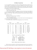
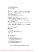
</div><span class="text_page_counter">Trang 20</span><div class="page_container" data-page="20">

Figure . Production and prediction crop production of BGD14

The purpose of this code snippet is to predict crop yields for the upcoming years using a linear regression model.

From the graph above, we can see that the food production of 4 crops of Bangladesh in the period 2026 and 2028 will all have positive growth. Bangladesh's domestic agricultural output is not enough to meet domestic consumption demand. Therefore, they choose to import food from abroad and Vietnam is one of the countries Bangladesh chooses to cooperate with. The Minister of Food of Bangladesh said that the country's rice production is insufficient to supply 170 million people, so Bangladesh still needs to import rice from the main suppliers including Vietnam. For the Bangladesh market, VINAFOOD II has been the main supplier of rice under the MOU for many years now. Of which, 2011 provided 450,000 tons; in 2017 supply 250,000 tons; in 2021 supply 52,500 tons of white rice; and in 2022 supply 230,000 tons of rice. Also according to Bangladesh's Food Minister, the country's rice production is not enough to supply 170 million people, so Bangladesh still needs to import rice, with the main suppliers being India, Vietnam and Myanmar. In that spirit, Bangladesh has agreed to extend the MOU on rice trade with Vietnam for another five

</div><span class="text_page_counter">Trang 21</span><div class="page_container" data-page="21">

years.

Utilizing similar code lines in this section and extracting information from the data file, we can predict the agricultural yields of the next six countries.

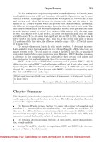
<b>7.2. China’s crop production (CHN) </b>

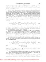
We will forecast the CHN's crop production including 4 crops and find the CHN's production forecast for the period between 2026 and 2028.

Figure 15. Production and prediction crop production of CHN

From the forecast chart, it can be seen that China's 4 crop food production -forecast for the period between 2026 and 2028, both recorded an increase. In 2022, China's total food production reached 686.55 million tons, up 3.7 million tons, equivalent to 0.5% compared to 2021, continuing to record a new record, maintaining production of more than 650 million tons, stable for 8 consecutive years. According to data released by the State Bureau of Statistics of China on December 12, the country's food production increased in all three harvests of the year. In terms of main foods, production of wheat and maize both increased slightly, rice decreased by 2%, and

</div>