project bank finance
Bạn đang xem bản rút gọn của tài liệu. Xem và tải ngay bản đầy đủ của tài liệu tại đây (6.08 MB, 39 trang )
<span class="text_page_counter">Trang 1</span><div class="page_container" data-page="1">
<b>FINAL PROJECT</b>
<i><b><small>Big Assignment (Official)</small></b></i>
<b><small>Program: VNUCourse Code: INS300801Course Title: Project</small></b>
</div><span class="text_page_counter">Trang 2</span><div class="page_container" data-page="2"><small>1.6. Project Contributions of each Member...5</small>
<b><small>2. Methodology and Solution...5</small></b>
<small>2.1. ARIMA...5</small>
<small>2.2. K- means...6</small>
<small>2.3. Apriori...7</small>
<b><small>3. Implementation and Results Analysis...8</small></b>
<small>3.1. Introducing the data:...8</small>
</div><span class="text_page_counter">Trang 3</span><div class="page_container" data-page="3">1.1 About the project
The topic we chose in this project is data analysis of an e-commerce fashion company in Indonesia called Fashion Campus. This company introduces domestic and international brands loved by young people. Our project focuses on analyzing the company's sales on the e-commerce platform to provide strategies for the company's departments.
1.2. Project Goals
This project also helps sellers on the Fashion Campus e-commerce platform refer to upcoming fashion trends. Hopefully our analytical models will help sales staff optimize performance and finances, accurately grasp customer psychology, to create the highest profits and revenue for businesses. Stakeholders of the Marketing Team and some of the Business Teams want to know the probability of users churning in the next one month. They also want to know how accurate our model is because this will influence the strategic decisions of the marketing team as well as the sales team. Thanks to that, businesses can confidently compete with other competitors.
1.3. Project Scope/ Out of scope
Analyze customer reviews, sales history data, pricing and promotions, market segmentation, and customer segmentation based on similar old products to evaluate and analyze customer needs as well as future market trends. We clearly define the product sector of the fashion e-commerce industry here, referring to the fashion industry segment based on price and quality, perhaps the main segment is the popular and teenagers. Out of Scope
The report's primary focus is on sales trends and consumer feedback so it does not delve into other product categories or business areas of the company and also does not address
</div><span class="text_page_counter">Trang 4</span><div class="page_container" data-page="4">Shopee's marketing strategies for the fashion sector, the specific brands or styles of shoes, or their supply chain and sourcing methods.
The report does not extensively cover the customer service processes or mechanisms in place for addressing consumer concerns, as it concentrates on sales predictions. And it doesn’t provide details on Shopee's overall financial performance, market capitalization, or share prices, as it centers around forecasting unit sales rather than financial data. 1.4. Project Risk
Some potential risks in this project include: - Fields fluctuates.
- Error in data.
- Changing customer preferences and trends. - Competition from rivals.
- Changes in online shopping behavior.
- To minimize risk, it is necessary to use robust data analytics, field monitoring, active engagement with customers, and continuous updates of the forecast model. 1.5. Project Deliverables
Deliverables used past sales data, seasonal trends, market dynamics, sentiment analysis and customer return behavior to accurately forecast Fashion's fashion sales Campus. This dashboard will allow users to explore sales trends, historical data, and sentiment analysis results easily, helping them make informed decisions.
The dashboard will present a comprehensive overview of the company's performance, including key business metrics such as total sales, revenue, margins, and customer
</div><span class="text_page_counter">Trang 5</span><div class="page_container" data-page="5">satisfaction scores. This comprehensive perspective will help Fashion Campus leadership quickly assess the health of their business.
The dashboard will display dynamic sales trends over different time periods, highlighting patterns, seasonal fluctuations, and emerging market trends. Users will have the ability to interact with these visualizations to better understand sales data.
Integrating sentiment analysis tools into dashboards will provide valuable insights into customer attitudes and opinions related to products. It will provide sentiment scores that reflect overall customer sentiment and specific feedback on different products. These insights can be used to improve products and marketing strategies.
1.6. Project Contributions of each Member
<b>2. Methodology and Solution</b>
We choose 3 algorithms ARIMA, K-means, Apriori to analyze and then come up with marketing strategies for departments. Using ARIMA for revenue forecasting, Apriori for product association calculation, and K-Means for customer clustering can collectively solve several key problems for a company, enhancing both its strategic decision-making and operational efficiency.
By implementing ARIMA for revenue forecasting, the Apriori algorithm for product association, and K-Means for customer clustering, a company can enhance its forecasting accuracy, marketing effectiveness, inventory management, and overall strategic planning, leading to improved business performance.
2.1. ARIMA
ARIMA (AutoRegressive Integrated Moving Average) models are effective in forecasting time series data like revenue. By analyzing past revenue data, it can predict future sales, helping in budget planning and resource allocation. Trend and Seasonality
</div><span class="text_page_counter">Trang 6</span><div class="page_container" data-page="6">Understanding: ARIMA can handle various patterns in data, such as trends and seasonal variations, providing a more accurate and nuanced forecast.
- Challenge: Revenue forecasts in the fashion industry always change every year, we can see the Covid 19 epidemic as a typical example, a time when people go out less and buying and selling activities take place online. network more
- Solution: We will use the Arima algorithm ((AutoRegressive Integrated Moving Average)) to analyze historical sales data, predict future trends, and make informed decisions about marketing and merchandising strategies. inventory.
ARIMA (AutoRegressive Integrated Moving Average): is a model used to model and predict time series. It combines three elements: autoregressive (AR), integrated autoregressive (I), and moving average (MA).
+ Strength: Predict time series with high accuracy. Works well with spatial time series data that are regular or can be transformed to become regular.
+ Weakness: It is necessary to choose the correct parameters to fit the data, which is sometimes quite difficult. Does not handle highly volatile time series well.
- Impact: Based on this, marketing or management teams will have a strategy to promote the company's image to develop faster; The inventory problem has also been very difficult in recent years, and revenue forecasts can solve the inventory problem for the company.
2.2. K- means
Segmenting customers into distinct groups based on purchasing behavior and preferences allows for more personalized and effective marketing campaigns. Understanding different customer segments can aid in tailoring products and services to meet the specific needs of
</div><span class="text_page_counter">Trang 7</span><div class="page_container" data-page="7">each group. By identifying key customer segments, resources can be allocated more efficiently, focusing on the most profitable or promising groups.
- Challenge: Solve the complexity of understanding customers' diverse preferences in fashion.
- Solution: Explain how Fashion Campus uses K-Means clustering to segment customers based on purchasing behavior, interests, and demographics, allowing for personalized marketing and product recommendations.
Kmeans is an unsupervised data clustering algorithm. It divides data points into groups (clusters) with similar characteristics.
+ Strength:
Efficient with big data and can help identify similar groups without labels. Easy to implement and suitable for data clustering when labels are not available.
+ Weakness:
The result depends heavily on the initial number of clusters (K). Does not always produce good clustering results, especially when the data does not divide clearly.
- Impact: This method will have many effects, such as increasing customer satisfaction, sharing incentives for different customers, loyalty and sales.
2.3. Apriori
The Apriori algorithm can reveal associations between different products purchased together. This insight is invaluable for cross-selling and upselling strategies. Inventory Management: Understanding product associations helps in managing inventory more effectively, ensuring that related products are adequately stocked.
</div><span class="text_page_counter">Trang 8</span><div class="page_container" data-page="8">- Challenge: Discuss the difficulty of determining which products are commonly purchased together.
- Solution: Describe how to use the Apriori algorithm to discover relationships between different fashion items, helping to create effective cross-selling and up-selling strategies. Apriori is an algorithm for mining association rules in purchase data. It detects relationships between items purchased together.
+ Strength: Detect common shopping patterns, helping businesses understand the relationship between items. Widely used in generating product recommendations based on previous purchase behavior.
+ Weakness:Does not handle data sets that are large or contain many items well (can cause performance issues). Requires time to calculate association rules, especially with large data.
-Impact: Show how analytics led to more strategic product placement and promotion, driving sales and customer engagement.
<b>3. Implementation and Results Analysis.</b>
3.1. Introducing the data:
The data set is taken from Fashion Campus, including demographic data, transactions and clicking data of e -commerce fashion company. Data fields are understood as follows:
- Data of Customer:
Customer_id Unique customer id first_name First of customer last_name Last name of customer
</div><span class="text_page_counter">Trang 9</span><div class="page_container" data-page="9">username User name of customer
gender Gender of customer (Male (M) or Female (F))
birthdate Birthdate of customer, day/month/year device_type Type of device
device_version Version of device
home_location_lat Latitude location of the customer home_location_long Customer's longitude location home_location Name of customer's province/region home_country Name of customer’s country first_join_date The first day customers join
- Data of Product:
gender Objective/Product Development masterCategory The main product category subCategory Subcategory of the product portfolio articleType Type fashion Products
baseColour Basic color of fashion products season Objective/Product Development based
on season
</div><span class="text_page_counter">Trang 10</span><div class="page_container" data-page="10">year Year production
usage Objective/Product Development based
customer_id The only ID of each customer booking_id The only ID of the transaction session_id The only session of the user when
accessing the application
product_metadata The metadata of the product has been purchased
payment_method Payment method is used in transactions payment_status Payment state (success/failure) promo_amount Promotional amount in each
transaction promo_code Promotion code
shipment_fee Shipping fee of transaction (Ongkir) shipment_date_limit Cardboard limit data
shipment_location_lat Location/latitude of shipment shipment_location_long Location of shipments
total_amount The total amount payable for each transaction
</div><span class="text_page_counter">Trang 11</span><div class="page_container" data-page="11">3.2. ARIMA:
Time series analysis is the process of studying and analyzing data over time to understand and expect trends, model and variations in series data. The ARIMA (AutoRegressive Integrated Moving Average) model is one of the popular time series analysis methods. The ARIMA model combines three main components: automatic recovery (automatic), moving average (moving average) and integrated analysis (integrated).
- Automatic process recovery (autoregression) (AR): Evaluates and predicts the current value of series data based on the previous value of that series. AR models use a numerical automatic recovery process to simulate dependencies between values in a sequence.
- Moving average (MA): Estimates and predicts the current value of series data based on averaging the most recent value observations. The MA model uses average parameters to simulate random variables in the series.
- Integral (integrate) (I): Adjusts series data to remove trends and non-random fluctuations. Analytical integration is used to convert unstable string data into string stable data.
The ARIMA model can be used to predict future values based on past surveys. Determining the appropriate parameters for an ARIMA model is often based on analysis and testing of sequence data, including models that determine the best testing parameters and optimization methods.
Time series analysis time series - ARIMA model to analyze monthly or weekly trends in total sales and seasonal patterns in product category sales. Objective: Estimate the company's revenue from which reasonable sales strategies can be devised => receive a total sales increase year by year, however by mid-2022 there will be signs of decline, Therefore, we focus on promoting marketing to increase purchasing revenue.
Analyze and visualize monthly sales trends from a single data transaction.
</div><span class="text_page_counter">Trang 12</span><div class="page_container" data-page="12">The chart shows a business's monthly sales trend over a year. Charts use trend lines to show the overall trend of the data.
Business sales tend to increase in the last months of the year. Sales are highest in December, the month before Christmas. The lowest sales were in March, the first month of the year.
Analyze and visualize weekly sales trends from transaction data sets.
This chart shows a retail business's sales by day of a week. Charts use trend lines to show the overall trend of the data.
In general, business sales tend to increase during the weekend and decrease during the middle of the week. Sales are highest on Friday, Saturday and Sunday. Sales are lowest on Mondays and Tuesdays.
● Weekly sales trend of a specific product over a year.
</div><span class="text_page_counter">Trang 13</span><div class="page_container" data-page="13">Apply the SARIMA model to the weekly sales forecasting problem
The SARIMA algorithm (Seasonal Autoregressive Integrated Moving Average) is a time series analysis and prediction algorithm. It is an extension of the conventional ARIMA model, specifically designed to handle seasonal data.
The trend element represents the increasing or decreasing momentum of the series in the future. For example, inflation is a general trend of economies, so the average price of the base basket of goods, also known as the CPI, always tends to increase and this upward trend represents a depreciation. of money.
Let's consider the Weekly Sales Trend graph of the trend factor in the time series of total sales
● We have a weekly sales trend based on the 'total_amount' column in the DataFrame df_transaction_trend.
df_transaction_trend.
</div><span class="text_page_counter">Trang 14</span><div class="page_container" data-page="14">We see that the series has a period of 1 year. The demand for shopping on e-commerce platforms increased in the months when the covid-19 epidemic began, when people stayed at home so shopping at home became more popular. In addition, we can use a seasonal decompose to extract the components that make up the series including: trend, season, residual like under:
So the components have been separated quite clearly as shown in the chart above. Next we will regress the SARIMA model.
● Dividing the train/test set First, to facilitate the validation of the forecasting model, we will divide the train/test set so that 2022 will be used as test data and the remaining data will be used for training. model training..
</div><span class="text_page_counter">Trang 15</span><div class="page_container" data-page="15">● We will examine the autocorrelation and partial correlation properties of the purchase series. From there, decide what range of values the autoregression and moving average of the ARIMA model should be in and use the stepwise method to find the most suitable model.
</div><span class="text_page_counter">Trang 16</span><div class="page_container" data-page="16">So from the chart we can choose the PACF partial autocorrelation and ACF
autocorrelation to be values less than or equal to 3. Because the series has a trend, we will take the first difference to create a stationary series, Or in other words, the degree of integration d = 1. In addition, we need to further determine the levels (P,D,Q) of the seasonal factor extracted from the original series. In order for the model to understand that we are regressing on the SARIMA model, we need to set the parameter
seasonal=True and the seasonal period m=12. The stepwise strategy will automatically find the best model based on the set parameters.
Using the stepwise method helps find the best SARIMA model. Performing stepwise search to minimize aic
ARIMA(0,1,0)(0,1,1)[12] : AIC=11956.349, Time=0.53 sec ARIMA(0,1,0)(0,1,0)[12] : AIC=12069.868, Time=0.07 sec ARIMA(1,1,0)(1,1,0)[12] : AIC=11926.986, Time=0.50 sec ARIMA(0,1,1)(0,1,1)[12] : AIC=11817.812, Time=0.57 sec ARIMA(0,1,1)(0,1,0)[12] : AIC=11914.806, Time=0.34 sec ARIMA(0,1,1)(1,1,1)[12] : AIC=11818.245, Time=1.15 sec ARIMA(0,1,1)(0,1,2)[12] : AIC=11818.294, Time=2.32 sec
</div><span class="text_page_counter">Trang 17</span><div class="page_container" data-page="17">ARIMA(0,1,1)(1,1,0)[12] : AIC=11847.335, Time=1.22 sec ARIMA(0,1,1)(1,1,2)[12] : AIC=11820.238, Time=3.94 sec ARIMA(1,1,1)(0,1,1)[12] : AIC=11817.415, Time=1.13 sec ARIMA(1,1,1)(0,1,0)[12] : AIC=11915.108, Time=0.60 sec ARIMA(1,1,1)(1,1,1)[12] : AIC=11817.288, Time=1.63 sec ARIMA(1,1,1)(1,1,0)[12] : AIC=11848.327, Time=1.65 sec ARIMA(1,1,1)(2,1,1)[12] : AIC=11819.288, Time=6.17 sec ARIMA(1,1,1)(1,1,2)[12] : AIC=11819.288, Time=4.44 sec ARIMA(1,1,1)(0,1,2)[12] : AIC=11817.340, Time=3.51 sec ARIMA(1,1,1)(2,1,0)[12] : AIC=11831.511, Time=2.88 sec ARIMA(1,1,1)(2,1,2)[12] : AIC=11820.650, Time=12.73 sec ARIMA(1,1,0)(1,1,1)[12] : AIC=11885.797, Time=1.40 sec ARIMA(2,1,1)(1,1,1)[12] : AIC=11819.210, Time=3.09 sec ARIMA(1,1,2)(1,1,1)[12] : AIC=11814.630, Time=5.08 sec ARIMA(1,1,2)(0,1,1)[12] : AIC=11814.776, Time=2.44 sec ARIMA(1,1,2)(1,1,0)[12] : AIC=11847.093, Time=1.18 sec ARIMA(1,1,2)(2,1,1)[12] : AIC=11816.629, Time=7.52 sec ARIMA(1,1,2)(1,1,2)[12] : AIC=11816.629, Time=8.56 sec ARIMA(1,1,2)(0,1,0)[12] : AIC=11914.927, Time=1.61 sec ARIMA(1,1,2)(0,1,2)[12] : AIC=11814.689, Time=4.57 sec ARIMA(1,1,2)(2,1,0)[12] : AIC=11829.594, Time=3.63 sec ARIMA(1,1,2)(2,1,2)[12] : AIC=11817.995, Time=6.24 sec ARIMA(0,1,2)(1,1,1)[12] : AIC=11812.895, Time=0.74 sec ARIMA(0,1,2)(0,1,1)[12] : AIC=11813.069, Time=0.52 sec ARIMA(0,1,2)(1,1,0)[12] : AIC=11845.262, Time=0.48 sec ARIMA(0,1,2)(2,1,1)[12] : AIC=11814.895, Time=2.06 sec ARIMA(0,1,2)(1,1,2)[12] : AIC=11814.895, Time=2.05 sec ARIMA(0,1,2)(0,1,0)[12] : AIC=11914.179, Time=0.22 sec ARIMA(0,1,2)(0,1,2)[12] : AIC=11812.949, Time=1.32 sec ARIMA(0,1,2)(2,1,0)[12] : AIC=11827.860, Time=1.07 sec ARIMA(0,1,2)(2,1,2)[12] : AIC=11816.239, Time=5.37 sec ARIMA(0,1,3)(1,1,1)[12] : AIC=11815.580, Time=1.61 sec ARIMA(1,1,3)(1,1,1)[12] : AIC=11817.575, Time=1.12 sec ARIMA(0,1,2)(1,1,1)[12] intercept : AIC=11822.842, Time=0.70 sec Best model: ARIMA(0,1,2)(1,1,1)[12]
Total fit time: 108.142 seconds
</div><span class="text_page_counter">Trang 18</span><div class="page_container" data-page="18">The stepwise method has helped us find the best SARIMA model for the forecasting problem as below:
● SARIMA model(p=0, d=1, q=2)(p=1, D=1, q=1, m=12). The model gives quite good results when the regression coefficients are all statistically significant (the entire P>|z| column is less than 0.05).
After finding the best ARIMA model. We will forecast for the next period. Forecasting for time series is quite specific and different from other classes of forecasting models because the previous time step value will be used to forecast the next time step. Therefore, a continuous loop of forecasting over time steps is required. Luckily, the
</div><span class="text_page_counter">Trang 19</span><div class="page_container" data-page="19">predict() function automatically helps us do that. We will only have to determine how many next sessions we want to forecast.
● forecast and visualize sales data for the next 12 months using the SARIMA model
The SARIMA model can predict future sales trends quite accurately. However, it should be noted that there may still be some random errors or sudden changes in sales trends.
● Seasonal patterns in product category sales.
</div>