ECO111_Microeconomics_All Chapter
Bạn đang xem bản rút gọn của tài liệu. Xem và tải ngay bản đầy đủ của tài liệu tại đây (9.47 MB, 104 trang )
<span class="text_page_counter">Trang 1</span><div class="page_container" data-page="1">
CHAPTER 1: 10 PRINCIPLES OF ECONOMIES
1. What Economics is all about?- Fundamental economic problem: The resources are scarce
- Scarcity: the limited nature of society’s resources When a society cannot produce all the goods and services people wish to have, it is said that the economy is experiencing scarcity
- Economics: the study of how society manages its scarce resources
2. How people make decisions:
a) Principle 1: People Face Tradeoffs - All decisions involve tradeoffs - Society faces an important tradeoff:
Efficiency: when society gets the most from its scarce resources
Equality: when prosperity is distributed uniformly among society’s members
Tradeoff: to achieve greater equality, could redistribute income from wealthy to poor. But this reduces incentive to work and produce, shrinks the size of the economic “pie”
Ex: Tax dollars paid by wealthy Americans and then distributed to those less fortunate may improve equality but lower the return to hard work and therefore reduce the level of output produced by our resources
Recognizing that tradeoffs exist does not indicate what decisions should or will be made b) Principle 2: The cost of something is what you give up to get it
- Making decisions requires comparing the costs and benefits of alternative choice
- The opportunity cost of any item is whatever must be given up to obtain it It is the relevant cost for decision making
Ex: Học phí đang sử dụng có thể đem gửi ngân hàng để lấy lãi Chi phí hiện
Học phí đang sử dụng, tiếp tục sử dụng Sau này đi làm lương cao Chi phí ẩn c) Principle 3: Rational people think at the margin
- Economists generally assume that people are rational
- Rational people: systematically and purposefully do the best they can to achieve their objectives Ex 1: Consumers want to purchase the goods and services that allow them the greatest level of satisfaction given their incomes and the prices they face
Ex 2: Firm managers want to produce the level of output that maximises the profits the firms earn - Many decisions in life involve incremental decisions:
Make decisions by evaluating costs and benefits of marginal changes – small incremental adjustments to an existing plan
Rational decision maker take action only if: Marginal benefits > Marginal costs
Ex 1: Suppose that flying a 200 – seat plane across the country costs the airline $100,000, which means that the average cost of each seat is $500. Suppose that the plane is minutes from departure and a passenger is willing to pay $300 for a seat. Should the airline sell the seat for $300? Of course it should. In this case, the marginal cost of an additional passenger is very small
</div><span class="text_page_counter">Trang 2</span><div class="page_container" data-page="2"> Ex 2: Why is water so cheap while diamonds are expensive? The marginal benefit of a good depends on how many units a person already has. Because water is plentiful, the marginal benefit of an additional cup is small. Because diamonds are rare, the marginal benefit of an extra diamond is high
d) Principle 4: People respond to incentives
- Incentive: something that induces a person to act, the prospect of a reward or punishment Ex: When gas prices rise, consumers buy more hubrid cars and fewer gas guzzling SUVs When cigarette taxes increase, teen smoking falls
- Because rational people make decisions by weighing costs and benefits, their decisions may change in response to incentives:
When the price of a good rises, consumers will buy less of it because its cost has risen When the price of a good rises, producers will allocate more resources to the production of
the good because the benefit from producing the good has risen.
- Many public policies change the costs and benefits that people face. Sometimes policymakers fail to understand how policies alter incentives and behaviour and a policy may lead to unintended consequences.
3. How people interact:
a) Principle 5: Trade can make everyone better off
- Rather than being self – sufficient, people can specialize in producing 1 good or service and exchange it for other goods
- Countries also benefit from trade & specialization: Get a better price abroad for goods they produce
Buy other goods more cheaply from abroad than could be produced at home b) Principle 6: Markets are usually a good way to organise economic activity
- Market: a group of buyers and sellers (need not be in a single location) - “Organize economic activity” means determining:
What goods to produce How to produce them
How much of each to produce Who gets them
- A market economy allocates resources through the decentralized decisions of many households and firms as they interact in markets for goods and services
- Famous insight by Adam Smith in The Wealth of Nations (1776): Each of these households and firms acts as if “led by an invisible hand” to promote general economic well – being
- The invisible hand works through the price system:
The interaction of buyers and sellers determines prices
Each price reflects the good’s value to buyers and the cost of producing the good
</div><span class="text_page_counter">Trang 3</span><div class="page_container" data-page="3"> Although individuals are motivated by self – interest, an invisible hand guides this self – interest into promoting society’s economic well – being
- When a government interferes in a market and prevents price from adjusting, household and firm decisions become distorted
- Centrally planned economies failed because they did not allow the market to work c) Principle 7: Governments can sometimes improve economic outcomes
- The invisible hand will only work if the government enforces property rights Important role for governments
Property rights: the ability of an individual to own and exercise control over scarce resources (with police, courts)
Ví dụ: sở y tế đã can thiệp để “bình ổn giá thị trường” tại các nhà thuốc trong đợt covid 19 People are less inclined to work, produce, invest, or purchase if large risk of their property
being stolen
- There are 2 broad reasons for the government to interfere with the economy: The promotion of efficiency and equality
- Government policy can be most useful wen there is market failure:
Market failure: when the market fails to allocate society’s resources efficiently Causes:
Externalities: when the production or consumption of a good affects bystanders (pollution) Market power: a single buyer or seller has substantial influence on market price
(monopoly)
In such cases, public policy may promote efficiency
Government may alter market outcome to promote equity (but not always)
- If the market’s distribution of economic well – being is not desirable, tax or welfare policies can change how the economic “pie” is divided
4. How the economy works as a whole works:
a) Principle 8: A country’s standard of living depends on its ability to produce goods & services - Huge variation in living standards across countries and overtime:
Average income in rich countries is more than 10 times average income in poor countries The US standard of living today is about 8 times larger than 100 years ago
Changes in living standards over time are also great
- The most important determinant of living standards: productivity, the amount of goods and services produced per unit of labor input
- Productivity depends on the equipment, skills, and technology available to workers. Other factors (labor unions, competition from abroad) have far less impact on living standards.
Thus, policymakers must understand the impact of any policy on our ability to produce goods and services
</div><span class="text_page_counter">Trang 4</span><div class="page_container" data-page="4">b) Principle 9: Prices rise when the government prints too much money - Inflation: increases in the general level of prices in the economy
- In the long run, inflation is almost always caused by excessive growth in the quantity of money, which causes the value of money to fall
- The faster the government creates money, the greater the inflation rate/ When the government creates a large amount of money, the value of money falls, leading to price increases
c) Principle 10: Society faces a short – run tradeoff between inflation and unemployment
- In the short – run (1 – 2 years), many economic policies push inflation and unemployment in opposite directions
- Other factors can make this tradeoff more or less favorable, but the tradeoff is always present - Most economists believe that the short – run effect of a monetary injection is lower
unemployment and higher prices:
An increase in the amount of money in the economy stimulates spending and thus the demand of the quantity of goods and services sold in the economy. The increase in the number of goods and services sold will cause firms to hire additional workers
An increase in the demand for goods and services leads to raise prices over time Some economists question whether this relationship still exists?
- The short – run tradeoff between inflation and unemployment plays a key role in the analysis of the business cycle
Business cycle: fluctuations in economic activity, such as employment and production
- Policymakers can exploit this trade-off by using various policy instruments, but the extent and desirability of these interventions is a subject of continuing debate
</div><span class="text_page_counter">Trang 5</span><div class="page_container" data-page="5">CHAPTER 2: THINKING LIKE AN ECONOMIST
- Economists play 2 roles: Scientists – try to explain the world, and Policy advisors – try to improve it I. The Economist as Scientist:
1. Economist follow the Scientific Method:
- The Scientific Method: the dispassionate development and testing of theories about how the world works
- Data can be collected and analysed to evaluate theories
- Using data to evaluate theories is more difficult in economics than in physical sceince because economists are unable to generate their own data and must make do with whatever data are available
Thus, economists pay close attention to the natural experiments offered by history
- For example: an economist researcher has a research topic about management/ marketing. They have to find out the determinants of purchasing intention for organic foods Key concepts
Research unit: individual (gen Z) Research scope: HCM city
Research objective: Find out determinants of purchasing intetion for organic foods
Therefore, they have to find and read the Theory of Planned Behavior (TPB) and then read the Articles to develop the Hypotheses base on the Assumptions
(biến X1) Price (biến X2) Quality
(biến X3) Environmental awareness (biến X4) Green promotion
(biến X5) Healthy awareness
Purchasing intention (biến Y) Conceptual framework/ model - Data collection:
Questionaires
Survey > 350 (số lượng gen Z)
Sau khi có dữ liệu, dùng dụng cụ để phân tích dữ liệu data analysis có kết quả Fingdings Applications (áp dụng cho doanh nghiệp), policy markers (người làm về chính sách)
And then, test the hypotheses
2. Assumptions make the World easier to understand:
- Assumptions simplify the complex world, make it easier to understand
- For example, to undertand international trade, it may be helpful to start out assuming that there are only 2 countries in the world producing only 2 goods. Once we understand how trade would work between these 2 countries, we can extend our analysis to a greater number of countries and goods - 1 important role of a scientist is to understand which assumptions one should make
- Economists often use assumptions that are somewhat unrealistic but will have small effects on the actual outcome of the answer
</div><span class="text_page_counter">Trang 6</span><div class="page_container" data-page="6">3. Economists use economic models to explain the World around us: - Most economic models are composed of diagrams and equations
- The goal of a model is to simplify reality in order to increase our understanding. This is where the use of assumptions is helpful
a) Model 1: The Circular Flow Diagram
- Circular Flow Diagram: a visual model of the economy that shows how dollars flow through markets among households and firms
- This diagram is a very simple model of the economy (note that it ignores the roles of government and international trade):
There are 2 markets: the market for goods and services and market of production’s factors There are 2 decision – makers: households and firms
The inner loop represents the flows of inputs and outputs between households and firms The outer loop represents the flows of dollars between households and firms
This model is closed
The conclusion: Total income = Total spending
- Factors of production – the resources the economy uses to produce goods & services, including: Labor: lực lượng lao động là đến từ household
Land: hộ gia đình có đất cho thuê đất/ hoặc xây nhà cho thuê mặt bằng
</div><span class="text_page_counter">Trang 7</span><div class="page_container" data-page="7"> Capital: có nguồn vốn nhàn rỗi Góp vốn vào các doanh nghiệp (buildings & machines used in production)
Income: thu nhập của hộ gia đình > wages: lương theo giờ, theo ngày (vì có nhiều nguồn) Salary: lương hàng tháng
b) Model 2: The Production Possibilities Frontier
- PPF – đường giới hạn khả năng sản xuất: a graph that shows the combinations of output that the economy can possibly produce given the available factors of production and the available production technology
- For example: an economy that produces 2 goods (cars and computers)
If all resources are devoted to produce cars: the economy would produce 1000 cars and 0 computers
If all resources are devoted to produce computers: the economy would produce 3000 computers and 0 cars
More likely, the resources will be divided between the 2 industries. The feasible combinations of output are shown on the PPF
- Impossible > Efficient > Inefficient:
Because resources are scarce, not every combination of computers and cars is possible. Production at a point outside of the curve (C) is not possible given the economy’s current level of resources and technology Impossible = infeasible = unattainable
Production is efficient at points on the curve (A and B). This implies that the economy is getting all it can from the scarce resources it has available There is no way to produce more of one good without producing less of another
Production at a point inside the curve (D) is inefficient:
</div><span class="text_page_counter">Trang 8</span><div class="page_container" data-page="8"> This means that the economy is producing less than it can from the resources it has available
If the source of the inefficiency is eliminated, the economy can increase its production of both goods
- The PPF reveals Principle 1: People face tradeoffs
Suppose the economy is currently producing 600 cars and 2,200 computers
To increase the production of cars to 700, the production of computers must fall to 2,000 - Principle 2 is also shown on the PPF: The cost of something is what you give up to get it
The opportunity cost of increasing the production of cars from 600 to 700 is 200 computers Thus, the opportunity cost of each car is two computers
- The opportunity cost of a car depends on the number of cars and computers currently produced
- Economists generally believe that PPF often have this bowed – out shape because some resources are better suited to the production of cars than computers (and vice versa)
c) The PPF’s exercises: - Slope: độ dốc
Opportunitiy cost for 1 horizontal good is SLOPE vertical good Opportunity cost for 1 vertical good is 1/ SLOPE horizontal good - For example:
Straigh line:
SlopeBC = = = - 2 (dấu trừ đang thể hiện downward sloping đường dốc đi xuống) Opportunity cost for 1 car is 2 bikes
Opportunity cost for 1 bike 0.5 car
Opportunity cost for 100 cars is 200 bikes SlopeDF = = = - 2
Constant opportunity cost
<small>Slope = </small>
</div><span class="text_page_counter">Trang 9</span><div class="page_container" data-page="9"> Bow shaped:
SlopeAC = = = - 0.125
Opportunity cost for 1 toy is 0.125 calculator Opportunity cost for 1 calculator is 8 toys SlopeAD = = =
Increasing opportunity cost (Bowed outwar)
As the economy shifts resources from toys to calculators: PPF becomes steeper, opportunity cost of calculators increase
PPF is bow – shaped when different workers have different skills, different opportunity costs of producing one good in terms of the other. The PPF would also be bow – shaped when there is some other resource, or mix of resources with varying opportunity costs (different types of land suited for different uses)
- Note:
With additional resources or an improvement in technology The economy can produce more goods The PPF can shift parallel outward (Economic growth can be illustrated by an outward shift of the PPF)
Moving from a point in the PPF to a point in the PPF Have tradeoffs
Moving from a point not in the PPF to a poin in the PPF No tradeoffs, no opportunity cost, change = 0
The PPF illustrates the concepts of: Tradeoffs and opportunity sost Efficiency and inefficiency
Unemployment and economic growth 4. Microeconomics and Macroeconomics:
- Economics is studied on various levels:
Microeconomics: the study of how households and firms make decisions and how they interact in markets
Macroeconomics: the study of economy – wide phenomena, including inflation, unemployment, and economic growth
- Microeconomics and macroeconomics are closely intertwined because changes in the overall economy arise from the decisions of individual households and firms.
</div><span class="text_page_counter">Trang 10</span><div class="page_container" data-page="10">- Because microeconomics and macroeconomics address different questions, each field has its own set of models which are often taught in separate courses
5. FYI: Who studies economics?
- Economics can seem abstract at first, but it is fundamentally very practical and the study of economics is useful in many different career paths
- This box provides a sample of well – known individuals who majored in economics in college II. The Economists as Policy Adviser:
1. Positive versus Normative analysis:
- For example, a discussion of minimum – wage laws: Polly says, “minimum – wage laws cause unemployment”; Norma says, “The government should raise the minimum wage”
- Positive statements: claims that attempt to describe the world as it is
- Normative statement: claims that attempt to prescribe how the world should be
Much of economics is positive: it tries to explain how the economy works. But those who use economics often have goals that are normative: They want to understand how to improve the economy
Positive statements can be confirmed or refuted, normative statements cannot - In the News: Football Economics
Economists often offer advice to policymakers (including football coaches)
This is an article from The Washington Post that describes economist David Romer’s research on the tendency of NFL teams to punt more often than necessary
2. Economists in Washington:
- Economists are aware that tradeoffs are involved in most policy decisions
- The president receives advice from the Council of Economic Advisers (created in 1946)
- Economists are also employed by administrative departments within the various federal agencies such as the Department of Treasury, the Department of Labor, the Congressional Budget Office, and the Federal Reserve
- The research and writings of economists can also indirectly affect public policy. 3. Why Economists’ advice is not always followed?
- The process by which economic policy is made differs from the idealized policy process assumed in textbooks
- Economists offer crucial input into the policy process, but their advice is only a part of the advice received by policymakers
</div><span class="text_page_counter">Trang 11</span><div class="page_container" data-page="11">III. Why Economists disagree:
1. Differences in Scientific Judgments:
- Economists may disagree about the validity of alternative positive theories or about the size of the effects of changes in the economy on the behaviour of households and firms.
- Example: some economists feel that a change in the tax code that would eliminate a tax on income and create a tax on consumption would increase saving in this country. However, other economists feel that the change in the tax system would have little effect on saving behavior and therefore do not support the change.
2. Differences in Values: 3. Perception versus reality:
- While it seems as if economists do not agree on much, this is in fact not true. Table 1 contains 14 propositions that are endorsed by a majority of economists
- Almost all economists believe that rent control adversely affects the availability and quality of housing.
- Most economists also oppose barriers to trade.
</div><span class="text_page_counter">Trang 12</span><div class="page_container" data-page="12">CHAPTER 4: THE MARKET FORCES OF SUPPLY AND DEMAND
I. Market Structure:1. Markets and Competition:
- A market is a group of buyers and sellers of a particular product. Markets can take many forms and may be organized (agricultural commodities) or less organized (ice cream)
- A competitive market: a market in which there are so many buyers and so many sellers that each has a negligible effect on market price. Each buyer knows that there are several sellers from which to choose. Sellers know that each buyer purchases only a small amount of the total amount sold
2. Types of market: - Perfect competition:
Characteristics:
The goods being offered for sale are exactly the same IDENTICAL, no prominence (Note: “Identical” is for Competition, “Similar” is for Oligopoly)
The buyers and sellers are so numerous that no single buyer or seller has any effect over the market price
Because buyers and sellers must accept the market price as given, they are often called the Price taker
No barrier: no capital, no law, no relationship Easily enter and out the market
Less advertisement
We will start by studying perfect competition because:
Perfectly competitive markets are the easiest to analyse because buyers and sellers take the price as a given
Because some degree of competition is present in most markets, many of the lessons that ws learn by studying supply and demand under perfect competition apply in more complicated markets
- Monopolistic competition:
Fall between extremes of perfect competition and monopoly Many sellers, many buyers
</div><span class="text_page_counter">Trang 13</span><div class="page_container" data-page="13">Ví dụ như bạn muốn vào thị trường đồ ăn nhanh rất dễ, nhưng đồ ăn thì có cơng thức chế biến khác nhau, cửa hàng của bạn phải có điểm đặc biệt (cơng thức chế biến) khác với cửa hàng khác Differentation
Chính vì sự khác biệt đó mà khi mới vào thị trường được quyền tạo giá, nhưng ngắn hạn: shortrun là do về lâu về dài đối thủ có thể tìm ra cơng thức của bạn Khi đó bạn trở thành Price taker Short – term Market power
Many competitors - Oligopoly:
Fall between extremes of perfect competition and monopoly Few sellers
More Barriers: capital, law, relationship Ví dụ như thị trường hàng khơng ở Việt Nam Price maker as groups (luật ngầm, không phá giá)
- Distinguish Demand from Need and Want:
Need: nhu cầu thiết yếu để duy trì sự tồn tại Đói và cần ăn để no bụng Want: different relies on culture and tradition
Ví dụ: người Việt khi đói muốn ăn cơm, người Pháp khi đói muốn ăn bánh mì Demand: ability to pay
Ví dụ: muốn ăn cơm tấm 50k nhưng chỉ có 30k nên phải ăn cái khác b) Definition of Demand Schedule:
- P: Price
- Q<small>d</small>: Quantity demanded (bao gồm need/ want/ demand) The Qd of any good is the amount of the good that buyers are willing and able to purchase
</div><span class="text_page_counter">Trang 14</span><div class="page_container" data-page="14">- This table is called The Demand Schedule: a table that shows the relationship between the price of a good and the quantity demanded
- One important determinant of quantity demanded is the price of the product:
Qd is negatively related to price. This implies that the demand curve is downward sloping Law of demand: the claim that the Qd of a good falls when the price of the good rises, other
things equal (Start from the price first)
- The red line is called the Demand Curve: a graphical representation of the relationship between the price of a good and the quantity demanded
6. Market Demand versus Individual Demand:
- Market demand: is the sum of all of the individual demands for a particular good or service Ex: Suppose Helen and Ken are the only 2 buyers in the Latte market:
</div><span class="text_page_counter">Trang 15</span><div class="page_container" data-page="15">- The demand curves are summed horizontally – meaning that the quantities demanded are added up for each level of price
- The market demand curve shows how the total quantity demanded of a good varies with the price of the good, holding constant all other factors that affect how much consmers want to buy
7. Presentation template:
Higher in price: (P2 > P1) Qd decrease at each price level (Qd 2 < Qd 1) (Law of demand) Move along the demand curve: đi dọc theo đường cầu (from point A to point B)
Change in the prices just move along the demand curve (Don’t shift) 8. Shifts in the Demand Curve:
- Determinants (variables) can shift the D curve are:
Number of buyers: P không thay đổi, Qd Shift D curve to the right (Qd increase at each P level)
Number of buyers: P không thay đổi, Qd Shift D curve to the left Income:
Normal goods – hàng hóa thiết yếu
When income Qd for Normal goods D curve for Normal goods shift to the right Inferior goods – hàng hóa thứ cấp (low quality)
</div><span class="text_page_counter">Trang 16</span><div class="page_container" data-page="16">When income Qd for Inferior goods D curve for Inferior goods shift to the left Không được quyền chốt lại normal goods/ inferior goods là gì vì nó sẽ phụ thuộc vào thu
nhập của từng đối tượng Prices of related goods:
Substitutes – thay thế: 2 goods are substitutes if an increase in the price of 1 causes an increase in demand for the other
Ví dụ đi từ Hà Nội về HCM sẽ có 2 lựa chọn là máy bay (A) hoặc xe lửa (B). Nhưng vào dịp Tết giá vé máy bay tăng cao Hành khách sẽ lựa chọn đi xe lửa nhiều hơn
PA QdB D curve (B) shifts to the right
Complements – bổ sung: 2 goods are complements if an increase in the price of one causes a fall in demand for the other
Ví dụ có 2 bổ sung cho nhau là A – xăng dầu, B – car:
Khi P<small>A</small> tăng, ban đầu người ta sẽ có xu hướng hạn chế sử dụng B, nhu cầu mua xăng dầu giảm Q<small>dA</small>
Về lâu về dài nếu P<small>A</small> cứ tăng mãi, người ta sẽ có xu hướng khơng sử dụng B nữa Q<small>dB</small> Khi đó, xuất hiện đối tượng xe khác không sử dụng xăng dầu là C thay thế B: Q<small>dC</small> Tastes – thị hiếu: anything that cause a shift in tastes toward a good will increase demand for
that good and shift its D curve to the right
Ví dụ như Hiếu Thứ Hai vơ tình mang giày Thượng Đình rồi làm MV Ngay sau đó người ta đổ xơ đi mua giày Thượng Đình
Expectations:
Ví dụ: bạn vừa mới phỏng vấn xin việc xong và được nhận
Hiện tại bạn chưa có lương nên bạn mua hàng với giá rẻ. Nhưng khi bạn được nhận, bạn biết tháng sau bạn sẽ có lương nên bạn bắt đầu mua hàng với giá cao hơn vì bạn biết trong tương lai bạn sẽ chi trả được Qd
III. Supply:
1. The Supply Curve:
- The Supply Curve: The relationship between price and quantity supplied
- Quantity Supplied: the amount of a good that sellers are willing and able to sell
Qs is positively related to price. This implies that the supply curve will be upward sloping P increase Qs increase at each price level
Law of supply: the claim that, other things equal, the Qs of a good rises when the price of the good rises
- Supply Schedule: a table that shows the relationship between the price of a good and the Qs - Supply Curve: a graph of the relationship between the price of a good and the Qs
</div><span class="text_page_counter">Trang 17</span><div class="page_container" data-page="17">Price of Ice Cream Cone Quantity of Cones Supplied
- The market supply curve can be found by summing individual supply curves - Individual supply curves are summed horizontally at every price
- The market supply curve shows how the total Qs varies as the price of the good varies - Change in Price Move along the Supply Curve
3. Shifts in the Supply curve:
- Variables that can shift the S Curve:
Number of sellers increase Qs increase at each price level S curve shifts to the right Technology develop Qs increase at each price level S curve shifts to the right
Ex: USA has 50,000 hours of working. In the past, they can produce 500 computers. But when the technology has improved, they are now producing 1000 computers
Price of inputs:
Ex: Cùng lượng tiền mà mua được nhiều input hơn thì sản xuất ra được nhiều output hơn. Ví dụ có 100k mua đường để làm bánh, bịch đường bình thường có giá 10k Mua được 10 bịch. Sau này bịch đường chỉ còn 8k Mua được 12 bịch đường Nhiều nguyên liệu hơn, sản xuất được nhiều bánh hơn. Do đó suy ra giá input giảm Lượng input tăng Output tăng theo
Expectations about the Future:
Ex: Ví dụ như bạn biết trong tương lai sản phẩm đó sẽ bị khan hiếm nguồn cung, trong khi demand vẫn giữ nguyên Trong tương lai, giá của sản phẩm đó sẽ tăng. Vậy nên hiện tại, bạn bắt đầu trữ hàng trong kho để bán trong tương lai, thì giá của sản phẩm ở hiện tại sẽ giảm
IV. Supply and Demand Together: 1. Equilibrium:
- The point where the supply and demand curves intersect is called the market’s equilibrium - Equilibrium: a situation in which the market price has reached the level at which Qs equals Qd - Equilibrium price: The price that balances Qs and Qd The equilibrium price is often called the
market – clearing price because both buyers and sellers are satisfied at this price - Equilibrium quantity: the Qs and the Qd at the equilibrium price
</div><span class="text_page_counter">Trang 18</span><div class="page_container" data-page="18">- If the actual market price is higher than the equilibrium price, there will be a surplus of the good Surplus: a situation in which Qs is greater than Qd
To eliminate the surplus, producers will cut the price until the market reaches equilibrium - If the actual price is lower than the equilibrium price, there will be a shortage of the good
Shortage: a situation in which Qd is greater than Qs
Sellers will respond to the shortage by rising the price of the good until the market reaches equilibrium
- Law of Supply and Demand: the claim that the price of any good adjust to bring the supply and demand for that good into balance
2. Three steps to analyzing changes in equilibrium:
- Decide whether the event shifts the supply or demand curve (or perhaps both) - Determine the direction in which the curve shifts: left or right
- Use the supply and demand diagram to see how the shift changes the equilibrium price and quantity Find the new Equilibrium
3. Shifts in Curves versus Movements along Curves:
- A shift in the demand curve is called a change in demand. A shift in the supply curve is called a change in supply
- A movement along a fixed demand curve is called a change in the quantity demanded. A movement along a fixed supply curve is called a change in the quantity supplied.
V. Conclusion: How prices allocate resources
- The model of supply and demand is a powerful tool for analysing markets
- Supply and demand together determine the prices of the econom’s goods and services: These prices serve as signals that guide the allocation of scarce resources in the economy Prices determine who produces each good and how much of each good is produced
</div><span class="text_page_counter">Trang 19</span><div class="page_container" data-page="19">VI. Exercises:
1. Case A: Numbers of sellers increase
- (1) Numbers of sellers increase Qs increases at each Price level The Supply curve shifts to the right from S1 to S2
- (2) At new equilibrium (S2 and D1): PE decrease (PE2 < PE1)
QE increase (QE2 > QE1)
2. Case B: Tastes change toward the positive direction
- (1) Tastes change toward the positive direction Means that people want to buy more at each price level Qd increase at each price level D curve shifts to the right from D1 to D2
- (2) At new equilibrium (S1 and D2): PE increase (PE2 > PE1)
QE increase (QE2 > QE1)
3. Case C: Inputs cost decrease and Income increase (Normal goods)
- (1) Inputs cost decrease Qs increases at each price level S curve shifts to the right from S1 to S2
</div><span class="text_page_counter">Trang 20</span><div class="page_container" data-page="20">- (2) In come increase (Normal goods) Qd increases at each price level D curve shifts to the right from D1 to D2
- (3) Conclusion: PE ambigous, QE increase 4. Case D:
Case E:
</div><span class="text_page_counter">Trang 21</span><div class="page_container" data-page="21">CHAPTER 5: ELASTICITY AND ITS APPLICATION
I. The Elasticity of Demand:1. Definition of elasticity:
- Elasticity: a measure of the responsiveness of Qd or Qs to one of its determinants
Elasticity: a measure of how much buyers and sellers repond to changes in market conditions 2. The Price Elasticity of Demand and its Determinants:
- Price elasticity of demand (PED): a measure of how much the Qd of a good responds to a change in the price of that good, computed as the percentage change in quantity demanded divided by the percentage change in price.
<small>PED = </small> - Determinants of the PED:
Availability of Close Substitutes: the more substitutes a good has, the more elastic its demand Necessities versus Luxuries: necessities are more price inelastic
- Market: narrowly defined markets (ice cream) have more elastic demand than broadly defined markets (food)
- Time Horizon: goods tend to have more elastic demand over longer time horizons
3. Computing the PED:
- Example: the price of ice cream rises by 10% and quantity demanded falls by 20%. PED = <sup>%</sup>
<small>%</small> = 2
- Because there is an inverse relationship between price and Qd, the PED is sometimes reported as a negative number We will ignore the minus sign and concentrate on the absolute value of the elasticity.
4. The Midpoint Method: A better way to calculate percentage changes and Elasticities
- Because we use percentage changes in calculating the PED, the elasticity calculated by going from 1 point to another on a demand curve will be different from an elasticity calculated by going from the 2nd point to the first. This difference arises because the percentage changes are calculated using a different base A way around this problem is to use the midpoint method
- Using the midpoint method involves calculating the percentage change in either PED by dividing the change in the variable by the midpoint between the initial and final levels rather than by the initial level itself
<small>Midpoint Methot = </small>
</div><span class="text_page_counter">Trang 22</span><div class="page_container" data-page="22">- Purpose: The midpoint method shows that the value is unchange
- The minus sign of the output shows the negative relationship Remind the Law of Demand 5. The Variety of Demand Curves:
- Classification of Elasticity:
When the PED > 1, demand is defined to be elastic When the PED < 1, the demand is defined to be inelastic When the PED = 1, the demand is said to have unit elasticity
- In general, the flatter the demand curve that passes through a given point, the more elastic the demand - Extreme Cases:
When the PED = 0, the demand is perfectly inelastic and is a vertical line
When the PED = ∞, the demand is perfectly elastic and is a horizontal line Perfect Competition
6. Total Revenue and the PED:
<small>- </small> Total revenue (TR): the amount paid by buyers and received by sellers of a good, computed as the price of the good times the quantity soldd
<small>TR = P x Q </small>
- If demand is inelastic, the percentage change in price will be greater than the percentage change in Qd:
If price rises, Qd falls, and total revenue will increase (because the increase in price will be larger than the decrease in quantity demanded).
</div><span class="text_page_counter">Trang 23</span><div class="page_container" data-page="23"> If price falls, Qd rises, and total revenue will decrease (because the fall in price will be larger than the increase in quantity demanded)
- If demand is elastic, the percentage change in Qd will be greater than the percentage change in price: If price rises, quantity demanded falls, and total revenue will decrease (because the increase in
price will be smaller than the decrease in quantity demanded
If price falls, quantity demanded rises, and total revenue will increase (because the fall in price will be smaller than the increase in quantity demanded)
- If demand is unit elastic, the percentage change in price will be equal to the percentage change in Qd:
If price rises, Qd falls, and total revenue will remain the same (because the increase in price will be equal to the decrease in quantity demanded)
If price falls, Qd rises, and total revenue will remain the same (because the fall in price will be equal to the increase in quantity demanded)
7. Elasticity and Total revenue along a linear Demand Curve:
- The slope of a linear demand curve is constant but the elasticity is not: At points with a low price and a high Qd, demand is inelastic At points with a high price and a low Qd, demand is elastic - Total revenue also varies at each point along the demand curve
- Presentation Template: for proving that “The slope of a linear demand curve is constant but the elasticity is not”
</div><span class="text_page_counter">Trang 24</span><div class="page_container" data-page="24"> The Elasticity is not constant
8. Other Demand Elasticites:
- Income elasticity of demand (IED): a measure of how much the quantity demanded of a good responds to a change in consumers’ income, computed as the percentage change in Qd divided by the percentage change in income:
<small>IED = </small> <sup>%</sup> <small>%</small>
Normal goods have positive income elasticities (IED > 0) Inferior goods have negative income elasticities (IED < 0) Luxuries tend to have positive income elasticities (IED > 0)
Necessities tend to have negative income elasticities (IED < 0)
- Cross – price elasticity of demand (CPED): a measure of how much the Qd of 1 good responds to a change in the price of another good, computed as the percentage change in the Qd of the first good divided by the percentage change in price of the second good:
<small>CPED = </small><sup>%</sup> <small>%</small>
Substitute goods have positive cross – price elasticities (CPED > 0) Complement goods have negative cross – price elasticities (CPED < 0)
II. The Elasticity of Supply:
1. The Price elasticity of Supply and its Determinants:
</div><span class="text_page_counter">Trang 25</span><div class="page_container" data-page="25">- Price elasticity of supply (PES): a measure of how much the Qs of a good responds to a change in the price of that good, computed as the percentage change in Qs divided by the percentage change in price
- Determinants of the PES:
Flexibility of sellers: goods that are somewhat fixed in supply (beachfront property) have inelastic supplies
Time horizon: supply is usually more inelastic in the short run than in the long run 2. Computing the Price Elasticity of Supply:
3. The Variety of Supply Curves: - Classification of Elasticity:
When the PES > 1, supply is defined to be elastic When the PES < 1, the supply is defined to be inelastic When the PES = 1, the supply is said to have unit elasticity
- In general, the flatter the supply curve that passes through a given point, the more elastic the supply - Extreme Cases:
When PES = 0, the supply is said to be perfectly inelasticity and is a vertical line When PES = ∞, the supply is said to be perfectly elastic and is a horizontal line
- Because firms often have a maximum capacity for production, the elasticity of supply may be very high at low levels of Qs and very low at high levels of Qs
</div><span class="text_page_counter">Trang 26</span><div class="page_container" data-page="26">III. Applications of Supply, Demand, and Elasticity:
1. A good news for Farming be bad news for Famers?
- A new hybrid of wheat is developed that is more productive than those used in the past. What happens?
- Supply increases, price falls, and Qd rises
- If demand is inelastic, the fall in price is more than the increase in Qd and total revenue falls - If demand is elastic, the fall in price is less than the rise in Qd and total revenue rises
- In practice, the demand for basic foodstuffs (like wheat) is usually inelastic: This means less revenue for farmers
Because farmers are price takers, they still have the incentive to adopt the new hybrid so that they can produce and sell more wheat
This may help explain why the number of farms has declined so dramatically over the past two
</div><span class="text_page_counter">Trang 27</span><div class="page_container" data-page="27">- In the 1970s and 1980s, OPEC reduced the amount of oil it was willing to supply to world markets. The decrease in supply led to an increase in the price of oil and a decrease in quantity demanded. The increase in price was much larger in the short run than the long run. Why?
- The demand and supply of oil are much more inelastic in the short run than the long run. The demand is more elastic in the long run because consumers can adjust to the higher price of oil by carpooling or buying a vehicle that gets better mileage. The supply is more elastic in the long run because non-OPEC producers will respond to the higher price of oil by increase more.
</div><span class="text_page_counter">Trang 28</span><div class="page_container" data-page="28">CHAPTER 6: SUPPLY, DEMAND AND GOVERNMENT POLICIES
I. Controls on Prices:1. Price floor and the way it affects Market Outcomes:
- Price floor: minimum A legal minimum on the price of a good or service - There are 2 possible outcomes if a price floor is put into place in a market:
If the price floor is less than or equal to the equilibrium price, it is not binding and has no effect on the price or quantity sold Legal
If the price floor is greater than the equilibrium price, it is a binding constraint and a surplus is created Illegal
- Case study: The minimum wage
The market for labor looks like any other market: downward – sloping demand, upward – sloping supply, an equilibrium price (called a wage), and an equilibrium quantity of labor hired
If the minimum wage is above the equilibrium wage in the labor market, a surplus of labor will
2. Price ceiling and the way it affects market outcomes:
- Price ceiling: maximum A legal maximum on the price of a good or service - There are 2 possible outcomes if a price ceiling is put into place in a market:
If the price ceiling is higher than or equal to the equilibrium price, it is not binding and has no effect on the price or quantity sold Legal
If the price ceiling is lower than the equilibrium price, it is a binding and shortage is created Illegal
</div><span class="text_page_counter">Trang 29</span><div class="page_container" data-page="29">- If a shortage for a product occurs and price cannot adjust to eliminate it, a method for rationing the good must develop
- Not all buyers benefit from a price ceiling because some will be unable to purchase the product
3. Evaluating Price controls:
- Because most economists feel that markets are usually a good way to organise economic activity, most oppose the use of price ceilings and floors:
Prices balance supply and demand and thus coordinate economic activity
If prices are set by laws, they obscure the signals that efficiently allocate scarce recources - Price ceilings and price floors often hurt the people they are intended to help:
Rent controls create a shortage of quality housing and provide disincentives for building maintenance
Minimum wage laws create higher rates of unemployment for teenager and low skilled workers II. Taxes:
1. How taxes on sellers affect market outcomes?
- If the government requires the seller to pay a certain dollar amount for each unit of a good sold, this will cause a decrease in supply
- The supply curve will shift upward by the amount of the tax - The quantity of the good sold will decrease
- Buyers and sellers will share the burden of the tax; buyers pay more for the good (including the tax) and sellers receive less
- 2 lessons can be learned here:
Taxes discourage market activity Buyers and sellers share burden of tax
</div><span class="text_page_counter">Trang 30</span><div class="page_container" data-page="30">2. How taxes on buyers affect market outcomes?
- If the government requires the buyer to pay a certain dollar amount for each unit of a good purchased, this will cause a decrease in demand
- The deman curve will shift downward by the amount of the tax - The quantity of goods sold will decrease
- Buyers and sellers will share the burden of the tax; buyers pay more for the good and sellers receive less
3. Elasticity and Tax incidence:
- Tax incidence: the manner in which the burden of a tax is shared among participants in a market - When supply is elastic and demand is inelastic, the largest share of the tax burden falls on buyers - When supply is inelastic and demand is elastic, the largest share of the tax burden falls on sellers - In general, a tax burden falls more heavily on the side of the market that is less elastic:
A small elasticity of demand means that buyers do not have good alternatives to consuming this product
A small elasticity of supply means that sellers do not have good alternatives to producing this particular good
</div><span class="text_page_counter">Trang 31</span><div class="page_container" data-page="31">- Case study: Who pays the luxury tax?
In 1990, Congress adopted a new luxury tax
The goal of the tax was to raise revenue from those who could most easily afford to pay
Because the demand for luxuries is often relatively more elastic than supply, the burden of the tax fell on suppliers and their workers
III. Presentation template: 1. Tax on sellers:
2. Tax on buyers:
3. Note:
- Both tax on buyers or sellers share the same burden
- But the burden not always $0.2 and $0.3, they will change depend on the slope and the elasticity IV. Exercises:
</div><span class="text_page_counter">Trang 32</span><div class="page_container" data-page="32">CHAPTER 7: CONSUMERS, PRODUCERS, AND THE EFFICIENCY OF MARKETS
<small>I. Definition of Welfare Economics: </small>
<small>- Welfare economics: the study of how the allocation of resources affects well – being</small>
<small>II. Consumer Surplus: </small>
<small>1. Willingness to Pay (WTP): </small>
<small>- WTP: the maximum amount that a buyer will pay for a good</small>
<small>- Consumer surplus (CS): the amount a buyer is willing to pay for a good minus the amount the buyer actually pays for it</small>
<small>- Total consumer surplus (TCS): sum of each buyer’s CS </small>
<small>CS = Value to buyers (WTP) – Amount paid by buyers TCS = CS of buyer 1 + CS of buyer 2 + … + CS of buyer n </small>
<small>Ở mức giá 70, CS của John tăng lên 30, còn tăng thêm là 10 </small>
</div><span class="text_page_counter">Trang 33</span><div class="page_container" data-page="33"><small>2. Using the Demand Curve to Measure CS: </small>
<small>- We can use the information on WTP to derive a demand curve </small>
<small>- At any given quantity, the price given by the demand curve reflects the WTP of the marginal buyer. Because the demand curve shows the buyer’s WTP, we can use the demand curve to measure CS </small>
<small>- CS can be measured as the area below the demand curve and above price </small>
<small>3. How a lower price raises CS? </small>
<small>- As price falls, CS increase for 2 reasons: </small>
<small> Those already buying the product will receive additional CS because they are paying less for the product than before </small>
<small> Because the price is now lower, some new buyers will enter the market and receive CS on these additional units of output purchased </small>
</div><span class="text_page_counter">Trang 34</span><div class="page_container" data-page="34"><small>4. What does CS measure? </small>
<small>- Remember that CS is the difference between the amount that buyers are willing to pay for a good and the price that they actually pay </small>
<small>- Thus it measures the benefit that consumers receive from the good as the buyers themselves perceive it Measure the economic well – being of consumers </small>
<small>III. Producer Surplus: </small>
<small>1. Cost and the Willingness to sell (WTS): </small>
<small>- Cost (WTS): the value of everything a seller must give up to produce a good </small>
<small>- PS: the amount a seller is paid for a good minus the seller’s cost of providing it - Total producer surplus (TPS): sum of each sellers’PS </small>
<small>PS = Amount received by sellers – Cost to sellers (WTS) TPS = PS of seller 1 + PS of seller 2 + … + PS of seller n </small>
<small>2. Using the Supply curve to mease Producer Surplus (PS): </small>
<small>- We can use the information on cost (WTS) to derive a supply curve </small>
</div><span class="text_page_counter">Trang 35</span><div class="page_container" data-page="35"><small>- At any given quantity, the price given by the supply curve represents the cost of the marginal seller. Because the supply curve shows the seller’s cost (WTS), we can use the supply curve to measure PS </small>
<small>- PS can be measured as the area above the supply curve and below the price </small>
<small>3. How a higher price raises PS? </small>
<small>- As price rises, PS increase for 2 reasons: </small>
<small> Those already selling the product will receive additional PS because they are receiving a higher price for the product than before </small>
<small> Because the price is now higher, some new sellers will enter the market and receive PS on these additional units of outpur sold </small>
<small>TPS at P2 is ADP 4. What does PS measure? </small>
<small>- PS is used to measure the economic well – being of producers IV. Market Efficiency: </small>
</div><span class="text_page_counter">Trang 36</span><div class="page_container" data-page="36"><small>1. The Benevolent Social Planner – Nhà hoạch định xã hội nhân từ: </small>
<small>- The economic well – being of everyone in society can be measured by total surplus (TS), which is the sum of CS and PS </small>
<small>TS = CS + PS </small>
<small>- Efficiency: the property of a resource allocation of maximising the TS received by all members of society - Equality: the property of distributing economic prosperity uniformly the members of society </small>
<small>2. Evaluating the Market equilibrium: - At the market equilibrium price: </small>
<small> Buyers who value the product more than the equilibrium price will consume the product; those who do not, will not buy the product. In other words, the free market allocates the supply of a good to the buyers who value it most highly, as measured by their WTP </small>
<small> Sellers whose costs are lower than the equilibrium price will produce the product; those whose are higher, will not sell the product. In other words, the free market allocates the demand for goods to the sellers who can produce it at the lowest cost </small>
<small>- TS is maximused at equilibrium price: </small>
<small> At any quantity of output smaller than the equilibrium quantity, the value of the product to the marginal buyer is greater than the cost to the marginal seller so TS would rise if output increases </small>
<small> At any quantity of output greater than the equilibrium quantity, the value of the product to the marginal buyer is less than the cost to the marginal seller so TS would rise if output decreases </small>
<small> This is one of the reasons that economists believe Principle 6: Markets are usually a good way to organise economic activity </small>
</div><span class="text_page_counter">Trang 37</span><div class="page_container" data-page="37"><small>Phần tam giác bên trái là deadweight loss V. Market Efficiency and Market Failure: </small>
<small>- To conclude that markets are efficient, we made several assumptions about how markets worked: Perfectly competitive markets </small>
<small> No extermalities </small>
<small>- When these assumptions do not hold, the market equilibrium may not be efficient - When markets fail, public policy can potentially remedy the situation </small>
<small>VI. Presentation template: 1. Exercise 1: </small>
<small>- For each of 3 potential buyers of oranges, the table displays the WTP for the first 3 oranges of the day. Assume Alex, Barb, and Carlos are the only 3 buyers of oranges, and only 3 oranges can be supplied per day </small>
<small>1st Orange 2nd Orange 3rd Orange </small>
</div><span class="text_page_counter">Trang 38</span><div class="page_container" data-page="38">CHAPTER 10: EXTERNALITIES
I. Externalities and Market Inefficienccy:- Market failure: is when the price mechanism leads to an inefficient allocation of resources and a deadweight loss of economic welfare (a net social welfare loss) Market failure exits when the competitive outcome of markets is not satisfactory from the point of view of society
- Key causes of Labour Market Failure: Labour Immobility:
Occupational immobility: barriers to moving easily between jobs
Geographical immobility: barriers to changing location to find a new job Disincentives to find/ take work:
The unemployment trap: where economic incentives to take a job are poor The poverty trap: where there are disincentives to earn extra income Discrimination by employers:
This is a part explanation of the gender gap in pay and women in senior roles Discrimination badly affects wages and employment for affected groups
Monopsony power of employers: they can use their “buying power” in labour market to drive down wages
- Externality: the uncompensated impact of one person’s actions on the well – being of a bystander
- Because buyers and sellers neglect the external effects of their actions when deciding how much to demand or supply, the market equilibrium is not efficient when there are externalities Equilibirum fails to maximize the total benefit to society as a whole
Ex: Self – interested paper firms will not consider the full cost of the pollution they create in their production process, and consumers of paper will not consider the full cost of the pollution they contribute from their purchasing decisions The firms will emit too much pollution unless the government prevents or discourages them from doing so
1. Welfare Economics: A Recap
- Use the welfare economics from chapter 7 to analyze the specific market: the market for aluminum
- The D curve:
Reflects the value of aluminum to consumers, as measured by the prices they are willing to pay At any given Q, the height of D curve show the WTP of marginal buyer
- The quantity produced and consumed in the market equilibrium – QMARKET is efficient Maximizes the sum of PS and CS
</div><span class="text_page_counter">Trang 39</span><div class="page_container" data-page="39">_The Market for Aluminum_ 2. Negative Externalities:
- Private costs (internal costs): faced by the producer or consumer directly involved in a transaction
<small> Private benefit </small>
- External cost: occur when the activity of one agent has a negative effect on the well being of a third party External benefit
- Suppose that aluminum factories emit pollution: For each unit of aluminum produced:
The Social cost = Private costs of the aluminum producers + Costs to bystanders affected The Social cost curve is above the S curve because of the external costs Reflect the cost of
pollution emitted
The benevolent social planner would choose the level of aluminum production at which the D curve crosses the Social cost curve This is the optimal amount from the standpoint of society as a whole
QMARKET > QOPTIMUM because the market equilibrium reflects only the private costs of production The marginal consumer values aluminum < The social cost of producing it
Reduce production and consumption below the market equilibrium level raises total economic well – being
- How to achieve the optimal outcome?
1 way: Taxing the producers for each ton of aluminum sold The tax would shift the S curve upward
If the tax = the external cost of pollutants The new S curve would concide with the Social cost curve
</div><span class="text_page_counter">Trang 40</span><div class="page_container" data-page="40">- The use of such a tax is called – Internalizing the externality: altering incentives so that people take account of the external effects of their actions
- Applying Principle 4: People respond to incentives
- Applying Principle 7: Governments can sometimes improve economic outcomes
_Pollution and the Social Optimum_ 3. Positive Externalities:
- Considering Education:
A more educated population leads to more informed voters Better government for everyone A more educated population tends to mean lower crime rates
A more educated population encourage the development and dissemination of technological advances Higher productivity and wages for everyone
- Social value > Private value The social value curve intersect S curve QOPTIMAL > QMARKET
_Education and the Social Optimum_
</div>