report 2 and 3 application of matlab in stability and quality of the system
Bạn đang xem bản rút gọn của tài liệu. Xem và tải ngay bản đầy đủ của tài liệu tại đây (4.61 MB, 52 trang )
<span class="text_page_counter">Trang 1</span><div class="page_container" data-page="1">
<b>HO CHI MINH UNIVERSITY OF TECHNOLOGY AND EDUCATION FACULTY OF INTERNATIONAL EDUCATION</b>
<b>REPORT 2 and 3: APPLICATION OF MATLAB IN STABILITY AND QUALITY OF THE SYSTEM</b>
<b>SUBJECT: AUTOMATIC CONTROL SYSTEMS IN PRACTICCOURSE ID: PACS320246E</b>
<b>Lecturer: MSc. Nguyễn Trần Minh Nguyệt</b>
<b>Student ‘s name- ID number: Võ Hoàng Việ – 21151436t </b>
<b> Nguyễn Trần Thanh Thủy-21151433</b>
</div><span class="text_page_counter">Trang 2</span><div class="page_container" data-page="2"><b>I.APPLICATION OF MATLAB IN STABILITY OF THE SYSTEM </b>
1. Investigation of a unit negative feedback system with an open-loop transfer function of G(s) by Bode Criterion.
b. Based on the Bode chart, find the gain crossover frequency, phase margin, phase crossover frequency and gain margin
c. Based on the Bode chart, find the gain crossover frequency, phase margin, phase crossover frequency and gain margin
d. Draw the transient response of the above system with unit step function as input for the time interval t=0÷10s to illustrate the conclusion in c. Save this drawing for
</div><span class="text_page_counter">Trang 3</span><div class="page_container" data-page="3"><b>b. Based on the Bode diagram, find Gain crossover ( </b><b> ) Phase crossover ( </b><b> ), Gain margin ( Gm) Phase margin , ( 𝐏𝐦) </b>
</div><span class="text_page_counter">Trang 4</span><div class="page_container" data-page="4"><i>Gain crossover (</i> <i>): </i>Locate the frequency at which the magnitude of the openloop transfer function is equal to 1 or 0 dB on the bode diagram According to Bode Diagram, we have = 0.45rad/s
<i>Phase crossover ( </i> <i>): </i>Locate the frequency at which the phase of the open-loop transfer function crosses -180
According to Bode Diagram, we have =4.64 rad/s
</div><span class="text_page_counter">Trang 5</span><div class="page_container" data-page="5">Add command margin(G)to the code, we have
Based on Bode Diagram, Gain crossover ( ) Phase crossover ( ), Gain margin ( Gm), Phase margin ( Pm) which calculated are roughly the same as using the
<b>d. Draw the transient response of the above system with the input as an internal unit step function time period t=0÷10s to illustrate the conclusion in question c </b>
</div><span class="text_page_counter">Trang 6</span><div class="page_container" data-page="6">The step response reaches and stays within 0.714% of its steady-state value. Hence the system is stable and the conclusion when using Bode diagram is right
</div><span class="text_page_counter">Trang 7</span><div class="page_container" data-page="7">Result:
<b>- Based on the Bode diagram, find the Gain crossover (</b><b> ) Phase crossover ( ) , Gain margin ( </b> <b>Gm), Phase margin ( 𝑷𝒎) </b>
</div><span class="text_page_counter">Trang 8</span><div class="page_container" data-page="8">Apply the same method question b we have:of , Gain crossover: = 6.64 rad/s
Phase crossover : = 4.67 rad/s
</div><span class="text_page_counter">Trang 9</span><div class="page_container" data-page="9"><b>- Draw the transient response of the above system with the input as an internal unit step function time period t=0÷10s </b>
Code:
</div><span class="text_page_counter">Trang 10</span><div class="page_container" data-page="10">Gk=feedback(G,1) step(Gk,10) Result:
Conclusion:
Increasing the K coefficient to 400 makes the transient response fluctuates larger and larger when it approaches 10s. Hence the system is stable and the un conclusion when using bode diagram right.is
<b>2. Investigation of a unit negative feedback system by Nyquist Criterion. 2.1. Investigate a unit negative feedback system with an open-loop transfer </b>
</div><span class="text_page_counter">Trang 11</span><div class="page_container" data-page="11">b. Based on the Nyquist chart, find the phase margin and gain margin (dB). c. Consider the stability of a closed system and explain
d. With K=400, repeat the requirements from a→c4
</div><span class="text_page_counter">Trang 12</span><div class="page_container" data-page="12">To find the Phase margin, we find the intersection point between the Nyqusist diagram and the unit circle O with radius is 1.
Phase Margin = 103 (deg)
To find gain Margin , we locate the phase crossing of the −180◦-line and draw a vertical line up to the corresponding magnitude plot. The distance between the 0-dB line and the magnitude plot is the gain margin.
Comment:
Compared to the result in request 2.1.2, both values of Gain Margin and Phase Margin are equal, regardless of using two types of graphs to demonstrate.
<b>c. Consider the stability of a closed system and explain </b>
-We first considerer values of poles of the opened-loop transfer function G. Matlab code:
G=tf([10], conv([1 0.2], [1 8 20])) pzplot(G)
Result:
</div><span class="text_page_counter">Trang 13</span><div class="page_container" data-page="13">All the poles lay on the negative side of Imaginary Axis, so the opened-loop transfer function G is stable.
-Secondly, we eventually define the stability of closed-loop transfer function G by relying on Nyquist graph of the opened-loop transfer function G.
Matlab code:
G=tf([10], conv([1 0.2], [1 8 20])) nyquist(G)
Result:
</div><span class="text_page_counter">Trang 14</span><div class="page_container" data-page="14">The Nyquist graph of the opened-loop transfer function G does not encircle the point (-1,0) in coordinate system.
<b>Conclusion: Combining two conditions (opened-loop transfer function G is stable and </b>
The Nyquist graph of it does not encircle the point (-1,0)), we jump to a conclusion that the closed-loop transfer function G is stable.
Comparing the value of Gain Margin and Phase Margin found from (b), both GM and PM are positive, so the closed-loop transfer function G is stable.
Therefore, in two ways to define the stability of the closed-loop transfer function G show us the same consequence that the closed-loop transfer function G is stable.
<b>e. With K=400, repeat the requirements from a→c -Draw the Nyquist plot of the system </b>
Matlab code:
G=tf([400], conv ([1 0.2], [1 8 20])) nyquist(G)
grid on
</div><span class="text_page_counter">Trang 15</span><div class="page_container" data-page="15">Result:
<b>- Based on the Nyquist chart, find the phase margin and gain margin (dB) </b>
</div><span class="text_page_counter">Trang 16</span><div class="page_container" data-page="16">Use method similar to answer 2.b, we have
Gain Margin : = − <small>−</small><sub></sub> = − <small>−</small><sub></sub> = − = − Phase Margin = -23.4 (deg)
=> Compared to the result in request 2.1.2, both values of Gain Margin and Phase Margin are equal, regardless of using two types of graphs to demonstrate.
<b>- Consider the stability of a closed system and explain </b>
We first considerer values of poles of the opened-loop transfer function G. Matlab code:
G=tf([400],conv([1 0.2],[1 8 20])) pzplot(G)
Result:
</div><span class="text_page_counter">Trang 17</span><div class="page_container" data-page="17">• The opened-loop transfer function G is stable because all the poles lay on the negative side of Imaginary Axis
Similarly, relying on Nyquist graph of the opened-loop transfer function G to find out the stability of closed-loop transfer function G.
</div><span class="text_page_counter">Trang 18</span><div class="page_container" data-page="18">• The Nyquist graph of the opened-loop transfer function G surrounds the point (-1,0) in coordinate system.
<b>Conclusion: Combining two conditions (opened-loop transfer function G is stable and </b>
The Nyquist graph of it surrounds the point (-1,0)), we jump to a conclusion that the closed-loop transfer function G is unstable.
Gain Margin and Phase Margin, which may be calculated from (b), both have negative values, indicating that the closed-loop transfer function G is unstable.
As a result, both definitions of the closed-loop transfer function G's stability led to the same conclusion: the function is unstable.
2.2. Consider the stability of a unit negative feedback system with an open-loop transfer function of:
</div><span class="text_page_counter">Trang 19</span><div class="page_container" data-page="19">• Two poles lay on the negative side of Imaginary Axis, and on poles at zero, so the opened-loop transfer function G(s) is stable.
<b>Nyquist graph of the opened-loop transfer function G(s): </b>
Matlab code:
G=tf([1],conv([1 1 0],[1 2])); nyquist(G)
Result:
</div><span class="text_page_counter">Trang 20</span><div class="page_container" data-page="20">• The Nyquist graph of the opened-loop transfer function G(s) does not encircle the point (-1,0) in coordinate system.
<b>Conclusion: The closed-loop transfer function G(s) is stable resulting from two </b>
consequences (the opened-loop transfer function G(s) is stable, and The Nyquist graph of it does not encircle the point (-1,0)).
<b>Using Bode diagram to make a comparation: </b>
</div><span class="text_page_counter">Trang 21</span><div class="page_container" data-page="21">
The values of Gain Margin and Phase Margin of the opened-loop transfer function are positive, so the closed-loop transfer function is stable.
Both ways expose the same result that the closed-loop transfer function is stable.
</div><span class="text_page_counter">Trang 22</span><div class="page_container" data-page="22">• The opened-loop transfer function G(s) is stable because one pole is located on the opposite side of the imaginary axis from the positive side and one pole at
</div><span class="text_page_counter">Trang 23</span><div class="page_container" data-page="23">• The point (-1,0) in the coordinate system is surrounded by the Nyquist graph of the opened-loop transfer function G.
<b>Conclusion: The closed-loop transfer function G is assumed to be unstable by combining </b>
two conditions: that the opened-loop transfer function G is stable and that its Nyquist graph surrounds the point (-1,0).
<b>Using Bode diagram to make a comparation: </b>
</div><span class="text_page_counter">Trang 24</span><div class="page_container" data-page="24">The closed-loop transfer function is unstable because the value of Gain Margin is infinite, and the value of Phase Margin is negative (the opened-loop transfer function). The closed-loop transfer function is unstable, and this is revealed in both ways.
<b>3. Implementation the system using Root Locus method </b>
Investigation the unit negative feedback system with an open-loop transfer function of G(s)
a. Draw the root locus of the system. Base on Root Locus to find K limit of the system, indicate this value on the figure.
b. Find K so that the system has a natural oscillation frequency ωn = 4 c. Find K so that the system has a damping coefficient = 0.7
d. Find K so that the system has an overshoot σmax% = 25% e. Find K so that the system has a settling time (2% standard) = 4s
<b>Solution in Matlab </b>
</div><span class="text_page_counter">Trang 25</span><div class="page_container" data-page="25"><b>a. Draw root locus of the system. Find K limit </b>
</div><span class="text_page_counter">Trang 26</span><div class="page_container" data-page="26">Hence K limit of the system is 174
<b>b. Find K to the system has natural oscillation frequency ωn = 4 </b>
In root locus, we have the decision poles: = − −
To Find K with ωn = 4, we find intersection of the root locus with circle with center O and radius 4 Choose the intersection near the virtual axis so that this K . value makes the system oscillate
</div><span class="text_page_counter">Trang 27</span><div class="page_container" data-page="27">Hence with frequency ωn = 4, K=8 and K=119
<b>c. Find K to the system has mping ξ = 0.7Da</b>
To find K with ξ = 0.7 we find the point that Damping is 0.7,
</div><span class="text_page_counter">Trang 28</span><div class="page_container" data-page="28">Hence with ξ = 0.7, The Gain K=23
<b>d. Find K to the system has Overshoot σmax% = 25% </b>
To σmax% = 25% we find the point which damping=0.404 ,
Hence the Gain K=43.6
<b>e. Find K to the system has settling time (2% standard) =4s </b>
</div><span class="text_page_counter">Trang 29</span><div class="page_container" data-page="29">
To find K when settling time equals to 4s, we find the intersection between the root locus and the straight line being parallel to the vertical axis cutting the
</div><span class="text_page_counter">Trang 32</span><div class="page_container" data-page="32"><b>Conclusion: Comparing the consequence of Matlab with the calculated result by </b>
Theory formulas, both of them are the same.
= =
</div><span class="text_page_counter">Trang 33</span><div class="page_container" data-page="33"><b>2.4. Analysis the control system by Root locus with transfer function </b>
a. Draw the Root Locus of the system. Base on Root Loucs, find K limit of the system, indicate this value on the figure. Save Root Locus as *.bmp file for reporting
b. Find K so that the system has a natural oscillation frequency ωn = 4 c. Find K so that the system has a damping coefficient ξ = 0.7 d. Find K so that the system has an overshoot σmax% = 25%
e. Find K so that the system has a settling time (standard 2%) = 4s. Investigate the above system using Bode and Nyquist diagrams when 𝐾 = 𝐾 limit/2
<b>Solution in Matlab </b>
<b>a. Draw the Root Locus of the system. Base on Root Loucs, find K limit of the system, indicate this value on the figure </b>
</div><span class="text_page_counter">Trang 34</span><div class="page_container" data-page="34">To find K limit, we find the intersection points between aginary is and Root LocusIm ax
</div><span class="text_page_counter">Trang 35</span><div class="page_container" data-page="35">K limit the system is of 103
<b>b. Find K so that the system has a natural oscillation frequency ωn = 4 </b>
To Find K with ωn = 4, we find intersection of the root locus with circle with center O and radius 4 Choose the intersection near the virtual axis so that this K . value makes the system oscillate
</div><span class="text_page_counter">Trang 36</span><div class="page_container" data-page="36">From the result, we have K=78.5
<b>c. Find K so that the system has a damping coefficient = 0.7</b> To find K with =0.7, we find the point at which Damping is 0.7
</div><span class="text_page_counter">Trang 37</span><div class="page_container" data-page="37">From Root Locus, there is no point whic damping coefficient = 0.7. Hence K h
To find K that σmax% = 25%, we find points which Damping equals to 0.404
From the result, we have K=9
<b>d. Find K so that the system has a settling time (2% standard) = 4s </b>
To find K when settling time equals to 4s, we find the intersection between the root locus and the straight line being parallel to the vertical axis cutting the horizontal axis at -1.
</div><span class="text_page_counter">Trang 38</span><div class="page_container" data-page="38">From the result, we have K=19
</div><span class="text_page_counter">Trang 43</span><div class="page_container" data-page="43"><b>Investigate the above system using bode and Nyquist plots when =Kgh/2</b>𝐾 The K limit of the system is 102
</div><span class="text_page_counter">Trang 44</span><div class="page_container" data-page="44">Result:
Comment:
Gain Margin Gm=6.06dB>0 Phase Margin Pm=38.5 deg>0 Hence the system is stable
<b>Using Nyquist Criterion: </b>
Apply Code:
G=tf([51 51], conv([1 5 0],[1 3 9])) nyquist(G)
grid on
</div><span class="text_page_counter">Trang 45</span><div class="page_container" data-page="45">Result:
Comment:
- No pole lying in the right-hand side of the complex plane – The Nyquist plot does not encircle the point (-1; j0) Hence the the close-loop system is stable by Nyquist criterion
<b>Open question: </b>
<b>1. Compare control system survey methods </b>
-Frequency method: Including Bode plot and Nyquist plot. Bode plots examine a system's frequency response and are often used to assess its stability and frequency performance. The Nyquist plot also shows frequency response information, but it uses a complicated graph that allows for the determination of system stability and transients.
</div><span class="text_page_counter">Trang 46</span><div class="page_container" data-page="46">-Feedback Metho Using Feedback from the system to evaluate its performance and d: stability. This method includes investigating the system's transfer function and inverse transfer function, as well as improving performance with tools such as PID tuning. -Timing method: In the time domain, it uses the input signal to measure the system's output signal. This method includes Time series analysis, time response graphs, and the application of Laplace transformation equations to determine system parameters
<b>2. When to use control system survey methods? </b>
-Frequency method: using in automatic control systems, electronics, and applications with high-frequency variations It allows for the evaluation of performance and stability at different frequencies.
-Feedback method Using to test the actual performance of the system under real : operating conditions, and when you need to adjust the controller to improve performance or ensure stability
-Timing method: Typically used in applications that require high real-time responses and control, such as robotics control and ship or aircraft control systems.
<b>3. Show the relationship between Bode and Nyquist plots. </b>
Both Bode and Nyquist plots provide information about a system's frequency response. The Bode plot represents the frequency response by representing the system's transfer function as a log-log plot with amplitudes and phase (oscillation) plots. Meanwhile, the Nyquist plot represents the frequency response using a complex graph, in which the real and imaginary parts of the transfer function are plotted on the complex plane
- The key relationship between these two graphs is that information from the Bode plot may be used to draw a Nyquist plot. The Bode plot can be used to detect frequency crossovers (oscillations) and phase offsets, which can determine the shape of the Nyquist plot and the system's stability.
</div><span class="text_page_counter">Trang 47</span><div class="page_container" data-page="47"><b>II. APPLICATION OF MATLAB IN QUALITY OF THE SYSTEM</b>
Investigate a unit negative feedback system with an open-loop transfer function of G(s)
a. With the K limit value found above, draw the transient response with the input as a unit step function. Verify that the output fluctuates?
b. With the K value found in question 3.3 d of experiment number 2, draw the transient response of the closed system with the input to the unit step function in the time range from 0 ÷ 5s. Find the overshoot and steady-state error of the system. Verify that the system has σmax% = 25%?
c. With the K value found in question 3.3 e of experiment number 2, draw the transient response of the closed system with the input to the unit step function in the time range from 0 ÷ 5s. Find the overshoot and steady-state error of the system. Verify that the system has txl = 4s?
d. Draw the two transient responses of questions b and c on the same figure. Note on the figure which response corresponds to that K
<b>Solution </b>
<b>a. With the K limit value found above, draw the transient response with the input as a unit step function. Verify that the output fluctuates? </b>
With K<small>limit </small>=173, substituting value of K<small>limit </small>into:
Matlab Code:
G=tf([173],conv([1 0.2],[1 8 20])) Gk=feedback(G,1)
step(Gk,50)
</div>