báo cáo bài quá trình 02 nhận dạng và điều khiển hệ thống
Bạn đang xem bản rút gọn của tài liệu. Xem và tải ngay bản đầy đủ của tài liệu tại đây (952.62 KB, 29 trang )
<span class="text_page_counter">Trang 1</span><div class="page_container" data-page="1">
BỘ GIÁO DỤC VÀ ĐÀO TẠOTRƯỜNG ĐẠI HỌC SƯ PHẠM KỸ THUẬT TP.
</div><span class="text_page_counter">Trang 2</span><div class="page_container" data-page="2">Tp. Hồ Chí Minh, tháng 6 năm 2023
Question 1:
Consider a spring-mass-dashpot system mounted on massless cart in Fig. 1. m=1kg is mass, k=0.1 is spring constant, =0.1 is friction coefficient,b u is the displacement of cart that is considered as an input, is they displacement of mass m that considered as output.
Figure 1.
a) Tìm mơ hình tốn của hệ thống dưới dạng phương trình khơng gian trạng thái.
Áp dụng định luật II Newton ta được:
</div><span class="text_page_counter">Trang 4</span><div class="page_container" data-page="4">- Ta nhấn “Run” để thực hiện lấy mẫu.
- Để kiểm chứng tại cửa sổ Command Window ta gõ “out.u” và “out.y”:
</div><span class="text_page_counter">Trang 5</span><div class="page_container" data-page="5">c) Khởi tạo một bộ thơng số m, k , b bất kì, thực hiện nhận dạng thông số hệ thống trên bằng Matlab/Simulink. - Tạo m file:
- Tạo file Simulink:
- Chọn “Parameter Estimator” Select Parameters
</div><span class="text_page_counter">Trang 6</span><div class="page_container" data-page="6">- Tích chọn như hình OK
OK
- Chọn “New Experiment”
</div><span class="text_page_counter">Trang 7</span><div class="page_container" data-page="7">- Chọn
OK
</div><span class="text_page_counter">Trang 8</span><div class="page_container" data-page="8">- Copy dữ liệu out.y
- Sau đó dán vào
</div><span class="text_page_counter">Trang 9</span><div class="page_container" data-page="9">Plot & Simulate
Estimate
</div><span class="text_page_counter">Trang 11</span><div class="page_container" data-page="11">EstimatedParams
- Hoặc chọn “Parameters”
</div><span class="text_page_counter">Trang 12</span><div class="page_container" data-page="12">- Thiết kế bộ điều khiển LQR:
+ Hàm tiêu chuẩn chất lượng có dạng:
</div><span class="text_page_counter">Trang 13</span><div class="page_container" data-page="13">+ Độ lợi hồi tiếp trạng thái: K R B P<small>1 T</small>
→ Luật điều khiển tối ưu:
- Thiết kế bộ điều khiển LQR trên Simulink:
</div><span class="text_page_counter">Trang 14</span><div class="page_container" data-page="14">e) Mô phỏng hệ thống bao gồm bộ điều khiển và nhận xét kết quả.
- Thời gian lấy mẫu là 0.01s. - Tín hiệu đặt là 100.
- Đáp ứng ngõ ra của hệ thống:
</div><span class="text_page_counter">Trang 15</span><div class="page_container" data-page="15">Fig.1 Model of the DC motor with the inertial load. The linear model of DC motor is
where <small>i</small>is the current, is the angular rate of the load, <small>vapp t( )</small>is the input voltage, and <small>y</small> is output. The parameters of the DC motor are <small>R2.0 [ ]W</small>,<small>L0.5 [ ]H</small>, <small>Km0.015 (torque constant)</small>,<small>Kb0.015 (emf constant)</small>,
<small>0.2 []</small>
<small>KNms</small>, <small>J0.02 [ .kg m2]</small>.
a) Tìm mơ hình tốn của hệ thống dưới dạng phương trình khơng gian trạng thái.
Mơ-men xoắn τ nhìn thấy ở trục động cơ:
τ(t) =i( )t
Điện áp tỷ lệ với tốc độ góc ω nhìn thấy ở trục:
=ω(t)
Phần điện:
→ ω( )t
</div><span class="text_page_counter">Trang 17</span><div class="page_container" data-page="17">Sơ đồ bên trong khối DC Motor:
</div><span class="text_page_counter">Trang 18</span><div class="page_container" data-page="18">- Ta nhấn “Run” để thực hiện lấy mẫu.
- Để kiểm chứng tại cửa sổ Command Window ta gõ “out.u” và “out.v”:
</div><span class="text_page_counter">Trang 19</span><div class="page_container" data-page="19">f) Khởi tạo một bộ thơng số bất kì, thực hiện nhận dạng thông số hệ thống trên bằng Matlab/Simulink.
- Tạo m file:
- Tạo file Simulink:
Sơ đồ bên trong khối DC Motor:
- Chọn “Parameter Estimator” Select Parameters
</div><span class="text_page_counter">Trang 20</span><div class="page_container" data-page="20">- Tích chọn như hình OK
OK
</div><span class="text_page_counter">Trang 21</span><div class="page_container" data-page="21">- Chọn “New Experiment”
- Chọn
</div><span class="text_page_counter">Trang 22</span><div class="page_container" data-page="22">OK
- Copy dữ liệu out.v
</div><span class="text_page_counter">Trang 23</span><div class="page_container" data-page="23">- Sau đó dán vào
Plot & Simulate
</div><span class="text_page_counter">Trang 24</span><div class="page_container" data-page="24">Estimate
</div><span class="text_page_counter">Trang 25</span><div class="page_container" data-page="25">EstimatedParams
- Hoặc chọn “Parameters”
</div><span class="text_page_counter">Trang 27</span><div class="page_container" data-page="27">R1 = 2.7426 →
; ; ;
- Thiết kế bộ điều khiển LQR:
+ Hàm tiêu chuẩn chất lượng có dạng: + Độ lợi hồi tiếp trạng thái: K R B P<small>1 T</small>
→ Luật điều khiển tối ưu:
- Thiết kế bộ điều khiển LQR trên Simulink:
</div><span class="text_page_counter">Trang 28</span><div class="page_container" data-page="28">h) Mô phỏng hệ thống bao gồm bộ điều khiển và nhận xét kết quả.
- Thời gian lấy mẫu là 0.01s. - Tín hiệu đặt là 100.
- Đáp ứng ngõ ra của hệ thống:
</div><span class="text_page_counter">Trang 29</span><div class="page_container" data-page="29">Độ vọt lố: 0%. Sai số xác lập là 0. Thời gian xác lập là 1.11s.
</div>