(Tiểu luận) survey and multivariate analysisind ividual portfolio
Bạn đang xem bản rút gọn của tài liệu. Xem và tải ngay bản đầy đủ của tài liệu tại đây (3.84 MB, 33 trang )
<span class="text_page_counter">Trang 1</span><div class="page_container" data-page="1">
<b>UNIVERSITY OF ECONOMICS HO CHI MINH CITYINTERNATIONAL SCHOOL OF BUSINESS</b>
<b>SURVEY AND MULTIVARIATE ANALYSIS</b>
</div><span class="text_page_counter">Trang 2</span><div class="page_container" data-page="2"><b>STUDENT SIGNATURE / DECLARATION</b>
<i>I declare that this submission is my own unaided work. It is being submitted inpartial fulfilment of the Survey and Multivariate Analysis unit.</i>
Lê Hoàng Đan Thanh
</div><span class="text_page_counter">Trang 3</span><div class="page_container" data-page="3">TABLE OF CONTENTS
1. Data “Repurchase intention”...xx
2. Data “Consumer satisfaction”...xx
3. Data “Consumer shopping well-being”...xx
4. Data “Performance”...xx
5. Data “Online shopping”...xx
6. Data “New product”...xx
7. Data “Buying car”...xx
8. Data “DataUEH”...xx
9. Data “UnichoiceLikert”...xx
10. Data “UnichoicePairedcomparison”...xx
“ProductDesign_plan” <i>“ProductDesign_prefs”...xx</i>
</div><span class="text_page_counter">Trang 4</span><div class="page_container" data-page="4">1. DATA “REPURCHASE INTENTION”
<b>1.1. The manager wishes to know which retailing website consumersmake purchase most frequently and least frequently. </b>
- To answer, we use Frequencies in Descriptive Statistics, then select “Web” in the other column.
+ Statistics Mode Continue
+ By Focusing on the Frequency column in the Frequency Table, we could see that ADAYROI and CHOTOT account for only 1% (as 1 would be in percentage)
- Result:
We could conclude that LAZADA has the highest purchase frequency with 44%, while ADAYROI and CHOTOT have the lowest with only 1%.
<b>1.2. In order to employ STP (segmenting – targeting – positioning), themanager wishes to know characteristics of the e-shopper in details(level of trust, gender, age, purchasing frequency, income and</b>
</div><span class="text_page_counter">Trang 5</span><div class="page_container" data-page="5">- With these numbers of Frequency, and the descriptive of:
</div><span class="text_page_counter">Trang 6</span><div class="page_container" data-page="6">Age of participants: 1 = under 25; 2 = 25 – 30; 3 = above 30
Purchase frequency of participants: 1 = once per month; 2 = twice per month; 3 = three times per month; 4 = four times or above per month
Monthly income of participants: 1 = under VND 5 million; 2 = VND 5 million - VND 10 million; 3 = above VND 10 million
Education level of participants : 1 = high school; 2 = college; 3 = university or higher
Trust in online shopping: 1 = low trust, 2 = medium trust, 3 = high trust => Consumers are predominantly female, mostly under 25, have medium-to-high trust in e-commerce, monthly purchase frequency, university level education or higher, and 5 to 10 million VND income.
<b>1.3.Following the same procedures as 1.1, we will have these tablesin order to employ STP (segmenting – targeting – positioning).</b>
- Variables must be in “Likert scale”. - Analyze Scale Reliability Analysis. - Select WOM1 for Items.
- Model is Alpha click OK (Same goes for IQ and RP).
- The Cronbach Alpha for WOM is .932, IQ is .870 and RP is .820 respectively. Due to all cases being valid, it’s safe to assume that the internal consistency of Word
of Mouth is excellent, while Repurchase Intention and Information Quality are good.
<b>1.4. Before employing data analysis, the manager wishes to check thereliability of the scales measuring WOM, IQ and RP based onCronbach alpha.</b>
- Select WOM, IQ and RP into the right box after entering Descriptive Statistics in
</div><span class="text_page_counter">Trang 7</span><div class="page_container" data-page="7">- Select Mean, Median, Mode, Range, Standard Deviation, Skewness, and Kurtosis from the “Statistics..” Click OK.
<b>1.5. The manager wishes to identify basic statistical figures of WOM, IQand RP including mean, median, mode, range, standard deviation,skewness and kurtosis.</b>
- We can use one-sample t-test will be implemented to answer this question. As a result, we obtain
<b>1.6. The manager wishes to know how trust varies due to different levelof age, purchase frequency and income.</b>
- Analyze Descriptive Statistics Crosstabs
Move TRU to Row(s) Move Age to Column(s) OK
Most under-25-year-old participants have high trust in e-shopping while the trust of the 25-30 tends to reach just medium.
- Similar to Purchase frequency
The more the purchase frequency increases, the lower the trust is in online
</div><span class="text_page_counter">Trang 8</span><div class="page_container" data-page="8">- Similar to Income
A large number of people who have income within the range from 5-10M VND buy things online and have high trust in online shopping.
<b>1.7. The manager thinks that WOM may influence heavily on consumerin online purchase, the manager wishes to test the hypothesis statingthat mean of WOM in the population exceeds 5.</b>
<b>1.8. The managers think that male and female consumer may notsimilar in their repurchase intention. Thus, the manager wishes tocheck whether repurchase intention is statistically different or notacross gender.</b>
- We will use the Independent samples t-test
</div><span class="text_page_counter">Trang 9</span><div class="page_container" data-page="9"><i>2. DATA </i>“CONSUMER SATISFACTION”
<b>2.1.Does satisfaction vary due to consumers’ gender?</b>
- Reliability check:
+ Analyze Scale Reliability Analysis
+ Move SAT1, SAT2, SAT3, SAT4 to the Variables box
+ In the “Statistics” Check the “Scale if item deleted” this will provide additional information if an item is removed click OK
Look for Cronbach's alpha coefficient in the output, it is 0.796 which is higher than 0.7.
- Combining all the variables:
+ Transform Compute variable Set like the picture Ok - Analyzing:
+ Analyze Compare Means Choose One-Way ANOVA
+ In the "One-Way ANOVA" dialog box, select the “satisfaction” variable
</div><span class="text_page_counter">Trang 10</span><div class="page_container" data-page="10">+ Click on the Post Hoc Select LSD OK to run the analysis.
+ Result: sig. 0.036 < 0.05 (the significant level)
There are significant differences in the satisfaction of customers considering their gender.
<b>2.2.Does satisfaction vary due to consumers’ age?</b>
- Analyzing:
+ Analyze Compare Means Choose One-Way ANOVA
+ In the "One-Way ANOVA" dialog box, select the “satisfaction” variable as the dependent variable and the “age” variable as the factor.
+ Result: for Ages 2.0 and 3.0, sig. 0.03 < 0.05
there are significant differences between the satisfaction of customers
</div><span class="text_page_counter">Trang 11</span><div class="page_container" data-page="11"><b>2.3.Does satisfaction vary due to consumers’ education?</b>
- Analyzing:
+ Analyze Compare Means Choose One-Way ANOVA
+ In the "One-Way ANOVA" dialog box, select the “satisfaction” variable as the dependent variable and the “Edu” variable as the factor.
- Result:
</div><span class="text_page_counter">Trang 12</span><div class="page_container" data-page="12">. Data “Consumer shopping well-being” Questions:
<b>3.1. Does shopping well-being vary due to consumer income under thepotential effect of utilitarian value?</b>
- Computing variable: + Transform -> Compute variable
+ Computing the first variable: SWB (Shopping well-being)
SWB in the “Numeric Expression” box. + Choose function groups Statistical
+ Choose functions and Special Variables -> Mean -> OK + The same goes for UV named “UVmean”
+ Analyze -> General Linear Model -> Univariate
</div><span class="text_page_counter">Trang 13</span><div class="page_container" data-page="13">The significance of UVmean is 0 (<0.05)
The significance of consumer income is 0.166 (>0.05)
The unitarian value affects SWB.
There is not enough evidence to prove the relationship between income and SWB.
<b>3.2. Does shopping well-being vary due to consumer income under thepotential effect of hedonic value?</b>
- Computing variable: + Transform -> Compute variable
</div><span class="text_page_counter">Trang 14</span><div class="page_container" data-page="14">“Numeric Expression” box.
+ Choose function groups Statistical
+ Choose functions and Special Variables -> Mean -> OK - Analyzing:
+ Analyze -> General Linear Model -> Hedonic + Compute the variable in the right category -> click OK
The significance of HV is 0 (<0.05): HV influences SWB
The significance of consumer income is 0.025 (<0.05): Income significantly affects SWB.
Shopping well-being varies due to hedonic value (HV) and consumer income.
<b>3.3. Does shopping well-being vary due to consumer income under thepotential effect both utilitarian value and hedonic value?</b>
(steps are exactly like questions 3.1 & 3.2)
</div><span class="text_page_counter">Trang 15</span><div class="page_container" data-page="15">Significant Effects: UVmean and HVmean (p-values of 0.000) Non-Significant Effects: Income (p-value of 0.073)
=> The impact of at least one independent variable on the SWB mean is significant. => UVmean and HVmean have the highest individual effects.
=> Income may not have a significant impact.
<b>3.4. Does shopping well-being vary due to consumer income and genderunder the potential effect of utilitarian value and hedonic value?</b>
(steps are exactly like question 3.1 & 3.2) - Result:
</div><span class="text_page_counter">Trang 16</span><div class="page_container" data-page="16">UVmean and HVmean (p-values 0.000) Weak effects: Income (p-value 0.162)
Gender and Income & Gender interaction (p-values > 0.05) are non-significant.
=> UVmean and HVmean have the highest individual effects. => Income may have a weak impact.
=> Gender and Income & Gender interaction don’t significantly impact SWBmean.
. Data “Performance” Questions:
<b>4.1. Are there any relationships among EMP, SAL, TRA, EXP, MAS,SUP and HWL? Which of them are significant?</b>
- We use Correlation analysis
- Check assumptions
+ Analyze Regression Linear
+ Move EMP to the “Dependant” box; SAL, TRA, EXP, MAS, SUP, and HWL to the “Independent” box.
+ Click on Statistics Check the “Collinearity diagnostics” box Continue
+ Click on Plots → put residual values (*ZRESID) in the Y box, and predicted values (*ZPRED) in the X box select “normal probability” Continue OK
- Analyzing:
<b>+ In “Analysis” -> Select “Correlate” -> Select “Bivariate”.</b>
+ Move all variables including EMP, SAL, TRA, EXP, MAS, SUP, and HWL to the “Variables” box.
+ Select “Pearson”, “Two-tailed” and “Flag significant correlations” so that SPSS can mark the statistically significant correlations based on your chosen alpha level (usually
</div><span class="text_page_counter">Trang 17</span><div class="page_container" data-page="17">Result:
- EMP: With SAL, TRA, EXP, MAS, and SUP, EMP both have a significant < 0.05. It means that there is a dramatic effect between EMP and these factors. Particularly, r between EMP and these factors are 0.622, 0.665, 0.663, 0.668, and 0.094, which indicates there are strongly positive relationship between EMP and these factors. Meanwhile, the significance for EMP and HWL is 0.892 > 0.05, so the HWL does not have a strong effect on EMP. - SAL: For TRA, EXP, MAS, and SUP, SAL both have significance at 0 <
0.05, and r are 0.679, 0.661, 0.646, 0.179, which means that there are strongly positive effects between SAL and these factors. However, the significance between SAL and HWL is 0.184, which indicates that the HWL and SAL don't have a significant impact on each other.
- TRA: The significance between TRA and EXP, MAS, and SUP are both < 0.05, and r is 0.696, 0.707, 0.171, so it means that TRA and these factors have strongly positive effects on each other. Meanwhile, the significance between TRA and HWL is 0.258 > 0.05, so there is no relation between TRA and HWL.
- EXP: With MAS and SUP, EXP both has significance at 0, and r are 0.853 and 0.197, so it means that there are significantly positive effects between EXP and these factors. However, the significance for EXP and HWL is 0.065, which means that there is no strong relation between EXP and HWL. - MAS: The significance between MAS and SUP, HWL are both < 0.05, and r
are 0.194 and 0.098, so it indicates that MAS and SUP, HWL have a strongly
</div><span class="text_page_counter">Trang 18</span><div class="page_container" data-page="18">- SUP: for HWL, SUP has significance at 0 < 0.05 and r at 0.76, so there is a significant positive between HWL and SUP.
<b>4.2.The EMP is potentially influenced by both SAL and MAS. If this isthe case, to which extent the variation of EMP is uniquely due toSAL? And, uniquely due to MAS?</b>
- Analyzing:
+ Analyze Regression Linear
+ Move the variable EMP into the box “Dependent”, MAS, and SAL into the box labeled Independent(s).
+ In the "Statistics" dialog box, check the box for "R squared change" under "Model fit" to obtain the change in the R-square value.
+ Continue OK - Result:
</div><span class="text_page_counter">Trang 19</span><div class="page_container" data-page="19">To know exactly the extent to which variation of EMP is uniquely due to SAL and MAS, let’s calculate it using the value of part (or semipartial) correlation.
For SAL, square its part correlation 0.25 and then multiply with 100, we have the result of 6.25. This means that 6.25 of the variance in EMP is accounted for uniquely by SAL.
We will do the same for MAS. And then we have the result of 12.18, which means that 12.18% of the variance in EMP is uniquely due to MAS.
<b>4.3.Whether increasing salary is a good solution for improvingemployees’ performance? To which extent employees’ salarypredicts their performance?</b>
- Analyzing:
+ Analyze Regression Linear
+ Specify the variables: In the Linear Regression dialog box, move the SAL (salary) into the "Independent" box, and the EMP (performance) into the "Dependent(s)" box.
</div><span class="text_page_counter">Trang 20</span><div class="page_container" data-page="20">- Result:
Looking at the Unstandardized Coefficient column: we can see that EMP = 2.027 + 0.586SAL
=> If we increase the salary by 1 dollar, we will see an increase of 58.6% in employee performance Considerably good to increase the salary.
Approximately 38.7% of the variance in the dependent variable (performance ratings) can be explained by the independent variable(s) (salary) included in the regression model.
Employees' salary predicts their performance ratings to a moderate extent and it is good to some extent to increase the salary and salary can predict 43.7% of the performance.
Performance-based bonuses, salary increases, offer competitive salaries to attract high-performing individuals to recruit.
<b>4.4.Whether providing more supports from managers is a goodsolution for improving employees’ performance? Identify the extentto which employees’ performance is explained by managers’support?</b>
- Analyzing:
+ Analyze Regression Linear
+ Move MAS (manager support) into the Independent box and EMP (performance) into the Dependant(s) box. OK
- Result:
</div><span class="text_page_counter">Trang 21</span><div class="page_container" data-page="21">- Approximately only 0.9% of the variance in employees' performance can be explained by managers' support in the regression model. This suggests that managers' support has a very limited explanatory power in predicting employees' performance.
- The equation: EMP = 4.734 + 0.77SUP
=> Only a 7.7% increase in performance if we raise the support.
=> Not a good solution as other factors can provide a better boost in performance.
<b>4.5.Do salary, training, experience, managers’ support, managementstyle and heavy workload predict employees’ performance? Towhich extent employees’ performance is explained by all thesefactors? Among the influencing factors, which is the most and theleast important factor in determining employees’ performance?</b>
In this case, the R-value of 0.745 indicates a good level of prediction. This means that the independent variables can predict the outcome variable (EMP), and predict it pretty well.
R square (coefficient of determination) is 0.555, which means that all of our independent variables can explain 55.5% of the variance in our dependent variable EMP.
</div><span class="text_page_counter">Trang 22</span><div class="page_container" data-page="22">To know exactly the importance level of each predictor variable, we will look at its standardized coefficients (beta value). The predictor with the largest absolute beta value is considered the most important factor, and vice versa. So, as shown in the table, the most important predictor is TRA with 0.269, and the least important factor is HWL with 0.021.
In conclusion, salary, training, experience, managers’ support, management style, and heavy workload do predict employees’ performance, and they can explain 55.5% of the variance in EMP. Also, the most and least important factors in determining EMP are TRA and HWL respectively.
5. Data “Online shopping” Questions:
<b>5.1.Which factors significantly explain for the differences between onlineshopping adopting group and online shopping refusing group?</b>
- Reliability check:
</div>