GroundbasedSARinterferometry:anoveltoolforGeoscience 1
GroundbasedSARinterferometry:anoveltoolforGeoscience
GuidoLuzi
X

Ground based SAR interferometry:
a novel tool for Geoscience

Guido Luzi
University of Florence
Italy

1. Introduction

The word Radar is the acronym of Radio detection and ranging. Radar is an active
instrument, which measures the echo of scattering objects, surfaces and volumes illuminated
by an electromagnetic wave internally generated belonging to the microwave portion of the
electromagnetic spectrum. It was born just before the second world war for detecting and
ranging target for non-civilian scopes. In this case the requested spatial resolution was not
so challenging for the technology available that time. The opening of new technological
frontiers in the fifties, including the satellites and the space vehicles, demanded a better
spatial resolution for application in geosciences remote sensing (RS). Synthetic aperture
radar (SAR) technique was invented to overcome resolution restrictions encountered in
radar observations from space and generally to improve the spatial resolution of radar
images. Thanks to the development of this peculiar technique, the radar observations have
been successfully refined, offering the opportunity of a microwave vision of several natural
media. Nowadays SAR instruments can produce microwave images of the earth from space
with resolution comparable to or better than optical systems and these images of natural
media disclosed the potentials of microwave remote sensing in the study of the earth
surfaces. The unique feature of this radar is that it uses the forward motion of the spacecraft
to synthesize a much longer antenna, which in turn, provides a high ground resolution. The

satellite SEASAT launched in 1978 was the first satellite with an imaging SAR system used
as a scientific sensor and it opened the road to the following missions: ERS, Radarsat,
ENVISAT, JERS till the recent TerraSARX and Cosmo-SkyMED. The measurement and
interpretation of backscattered signal is used to extract physical information from its
scattering properties. Since a SAR system is coherent, i.e. transmits and receive complex
signals with high frequency and phase stability, it is possible to use SAR images in an
interferometric mode. The top benefit from microwave observations is their independence
from clouds and sunlight but this capability can weaken by using interferometric techniques.
Among the several applications of SAR images aimed at the earth surface monitoring, in the
last decades interferometry has been playing a main role. In particular, it allows the detection,
with high precision, of the displacement component along the sensor–target line of sight.
The feasibility and the effectiveness of radar interferometry from satellite for monitoring
ground displacements at a regional scale due to subsidence (Ferretti et al., 2001),
1
GeoscienceandRemoteSensing,NewAchievements2


earthquakes and volcanoes (Zebker et al., 1994 , Sang-Ho, 2007 and Massonnet et al. 1993
(a)) and landslides (Lanari et al., 2004 ; Crosetto et al., 2005) or glacier motion (Goldenstein
et al., 1993 ; Kenyi and Kaufmann, 2003) have been well demonstrated. The use of
Differential Interferometry based on SAR images (DInSAR) was first developed for
spaceborne application but the majority of the applications investigated from space can be
extended to observations based on the use of a ground-based microwave interferometer to
whom this chapter is dedicated. Despite Ground based differential interferometry
(GBInSAR) was born later, in the last years it became more and more diffused, in particular
for monitoring landslides and slopes.

After this introduction the first following sections of this chapter resume SAR and
Interferometry techniques basics, taking largely profit from some educational sources from
literature (Rosen 2000; Massonnet, 2003a; Askne, 2004, Ferretti, 2007). The following sections

are devoted to the GBInSAR and to three case studies as examples of application of the
technique.

2. General radar properties

2.1 The radar equation
Conventional radar is a device which transmits a pulsed radio wave and the measured time
for the pulse to return from some scattering object, is used to determine the range. The
fundamental relation between the characteristics of the radar, a target and the received signal,
is called the radar equation, a relationship among radar parameters and target characteristics.
Among the possible formulations we comment that indicated by the following expression:


(1)


where P
t
is the transmitted power, G
tx
and G
rx
are the transmitting and receiving gains of the
two antennas, with respect to an isotropic radiator, is the radar cross section, R the distance
from the target, is the pulse carrier wavelength. In (1) a factor which takes into account the
reduction in power due to absorption of the signal during propagation to and from the target
is neglected. This expression allows to estimate the power of the signal backscattered from a
target at a known range, at a specific radar system configuration. The minimum detectable
signal of a target, proportional to the received power P
R

, can be estimated knowing the
transmitted power, P
T
, the antennas’ characteristics and the system noise; of note that the
range strongly influences the strength of the measuring signal. A radar image consists of the
representation of the received signal in a two dimensional map, obtained through the
combination of a spatial resolution along two directions, namely range and azimuth or cross-
range, which correspond in a satellite geometry to cross-track and along the track directions.
Normally the radar transmitting and receiving antennas are coincident or at the same location:
in this case we speak about a monostatic radar and the measured signal is considered coming
from the backward direction. In (1) we introduced the radar cross section, the parameter that
describes the target behavior. The radar cross section of a point target is a hypothetical area
intercepting that amount of power which, when scattered isotropically, produces an echo
equal to P
R
as received from the object. Consequently  can be found by using the radar
 
4
3
2
4
R
GG
PP
rxtx
TR






equation and measuring the ratio P
R
/P
T
and the distance R, supposing the system parameters
 , G
tx
, G
rx
, are known. In RS we are interested in the backscatter from extended targets then
we normalize the radar cross section with respect to a horizontal unit area, and we define a
backscattering coefficient, 
0,
usually expressed in dB. This fundamental information recorded
by a radar is a complex number namely an amplitude and a phase value at a certain
polarisation, electromagnetic frequency and incidence angle (Ulaby et al., 1984). The complex
backscattering coefficient in SAR system is usually measured at four orthogonal polarisation
states. Normally these polarization states are chosen to be HH (horizontal transmission and
horizontal reception), HV (horizontal transmission and vertical reception) and analogously
VH and VV. In this chapter we only consider the case of a single linear polarization, usually
VV. Finally we remind that the Microwave portion of the electromagnetic spectrum is usually
subdivided in bands, and Remote Sensing instrumentation mainly operates at L, S, C, X, Ku
and Ka band, corresponding to the following intervals : L (1GHz-2GHz) S (2GHz-4GHz), C
(4GHz-8GHz), X (8GHz-12 GHz), Ku (12-18 GHz) and Ka (26.5GHz-40 GHz) spanning in
vacuum wavelengths from 30. cm to 8.mm. A radar signal is subject to a specific noise, due to
the echoes coming from different parts of a reflecting body within a resolution cell which will
have different phases and hence causing in the signal summation constructive or destructive
interference between the different components. The resulting noise-like behaviour is called the
speckle noise. To reduce the effect of speckle we may use filters. One way to reduce speckle is to

use multi look processing which improves the S/N but worsening the spatial resolution
(Curlander et McDonough, 1991). Temporal coherent averaging is possible in case of large
number of images as in the Ground Bsed SAR Ground Based SAR –
GBSAR case.

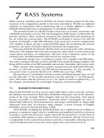
2.2 The range resolution
The range measurement is based on the fact that the signal echo is received after a delay of
T=2R/c, where R is the distance to the scattering object and c is the speed of the
electromagnetic pulse. In practice we use a pulse train where pulses are separated by a time
T
prf
,corresponding to a pulse repetition frequency, PRF = 1/T
prf
. This means that we have
an ambiguity problem: the measured radar echo can be caused by one pulse or the
subsequent. This translates in the following expression: PRF < c/2R
max
which relates the
maximum usable Range, R
max
, to PRF. The range resolution is determined by the pulse
width T of the pulse where the factor 2 is caused by the radar pulse going back and forth.
Figure 1 shows the working principle of range measurement through radar.


Fig. 1. The Radar functioning principle
GroundbasedSARinterferometry:anoveltoolforGeoscience 3


earthquakes and volcanoes (Zebker et al., 1994 , Sang-Ho, 2007 and Massonnet et al. 1993

(a)) and landslides (Lanari et al., 2004 ; Crosetto et al., 2005) or glacier motion (Goldenstein
et al., 1993 ; Kenyi and Kaufmann, 2003) have been well demonstrated. The use of
Differential Interferometry based on SAR images (DInSAR) was first developed for
spaceborne application but the majority of the applications investigated from space can be
extended to observations based on the use of a ground-based microwave interferometer to
whom this chapter is dedicated. Despite Ground based differential interferometry
(GBInSAR) was born later, in the last years it became more and more diffused, in particular
for monitoring landslides and slopes.

After this introduction the first following sections of this chapter resume SAR and
Interferometry techniques basics, taking largely profit from some educational sources from
literature (Rosen 2000; Massonnet, 2003a; Askne, 2004, Ferretti, 2007). The following sections
are devoted to the GBInSAR and to three case studies as examples of application of the
technique.

2. General radar properties

2.1 The radar equation
Conventional radar is a device which transmits a pulsed radio wave and the measured time
for the pulse to return from some scattering object, is used to determine the range. The
fundamental relation between the characteristics of the radar, a target and the received signal,
is called the radar equation, a relationship among radar parameters and target characteristics.
Among the possible formulations we comment that indicated by the following expression:


(1)


where P
t

is the transmitted power, G
tx
and G
rx
are the transmitting and receiving gains of the
two antennas, with respect to an isotropic radiator, is the radar cross section, R the distance
from the target, is the pulse carrier wavelength. In (1) a factor which takes into account the
reduction in power due to absorption of the signal during propagation to and from the target
is neglected. This expression allows to estimate the power of the signal backscattered from a
target at a known range, at a specific radar system configuration. The minimum detectable
signal of a target, proportional to the received power P
R
, can be estimated knowing the
transmitted power, P
T
, the antennas’ characteristics and the system noise; of note that the
range strongly influences the strength of the measuring signal. A radar image consists of the
representation of the received signal in a two dimensional map, obtained through the
combination of a spatial resolution along two directions, namely range and azimuth or cross-
range, which correspond in a satellite geometry to cross-track and along the track directions.
Normally the radar transmitting and receiving antennas are coincident or at the same location:
in this case we speak about a monostatic radar and the measured signal is considered coming
from the backward direction. In (1) we introduced the radar cross section, the parameter that
describes the target behavior. The radar cross section of a point target is a hypothetical area
intercepting that amount of power which, when scattered isotropically, produces an echo
equal to P
R
as received from the object. Consequently  can be found by using the radar
 
4

3
2
4
R
GG
PP
rxtx
TR





equation and measuring the ratio P
R
/P
T
and the distance R, supposing the system parameters
 , G
tx
, G
rx
, are known. In RS we are interested in the backscatter from extended targets then
we normalize the radar cross section with respect to a horizontal unit area, and we define a
backscattering coefficient, 
0,
usually expressed in dB. This fundamental information recorded
by a radar is a complex number namely an amplitude and a phase value at a certain
polarisation, electromagnetic frequency and incidence angle (Ulaby et al., 1984). The complex
backscattering coefficient in SAR system is usually measured at four orthogonal polarisation

states. Normally these polarization states are chosen to be HH (horizontal transmission and
horizontal reception), HV (horizontal transmission and vertical reception) and analogously
VH and VV. In this chapter we only consider the case of a single linear polarization, usually
VV. Finally we remind that the Microwave portion of the electromagnetic spectrum is usually
subdivided in bands, and Remote Sensing instrumentation mainly operates at L, S, C, X, Ku
and Ka band, corresponding to the following intervals : L (1GHz-2GHz) S (2GHz-4GHz), C
(4GHz-8GHz), X (8GHz-12 GHz), Ku (12-18 GHz) and Ka (26.5GHz-40 GHz) spanning in
vacuum wavelengths from 30. cm to 8.mm. A radar signal is subject to a specific noise, due to
the echoes coming from different parts of a reflecting body within a resolution cell which will
have different phases and hence causing in the signal summation constructive or destructive
interference between the different components. The resulting noise-like behaviour is called the
speckle noise. To reduce the effect of speckle we may use filters. One way to reduce speckle is to
use multi look processing which improves the S/N but worsening the spatial resolution
(Curlander et McDonough, 1991). Temporal coherent averaging is possible in case of large
number of images as in the Ground Bsed SAR Ground Based SAR –
GBSAR case.

2.2 The range resolution
The range measurement is based on the fact that the signal echo is received after a delay of
T=2R/c, where R is the distance to the scattering object and c is the speed of the
electromagnetic pulse. In practice we use a pulse train where pulses are separated by a time
T
prf
,corresponding to a pulse repetition frequency, PRF = 1/T
prf
. This means that we have
an ambiguity problem: the measured radar echo can be caused by one pulse or the
subsequent. This translates in the following expression: PRF < c/2R
max
which relates the

maximum usable Range, R
max
, to PRF. The range resolution is determined by the pulse
width T of the pulse where the factor 2 is caused by the radar pulse going back and forth.
Figure 1 shows the working principle of range measurement through radar.


Fig. 1. The Radar functioning principle
GeoscienceandRemoteSensing,NewAchievements4


The backscattered signal has an extension in time T due to the pulse width and in order to
obtain a good range resolution we need a short pulse. However, recalling Fourier transform
properties, a short pulse width means a large frequency bandwidth. At the same time as
dictated by the radar equation, at large distances, high amplitude is requested as the pulse
energy determines the detection possibilities of the system i.e. its signal to noise ratio (S/N).
This means that in designing a radar we are faced with the problem to want a long pulse
with high energy and a wide bandwidth which implies a short pulse. To reduce these
difficulties a signal processing technique, namely pulse compression, obtained by using a
“chirp radar” (Ulaby et al., 1982) can be used. In this case the transmitted frequency is
varying linearly with time and by correlating the return signal with a frequency modulated
signal, a sharp peak is obtained for a distance related to the time offset. The resolution
depends on the ability to sample sufficiently often the returned signals not to be aliased by
the sampling rate.

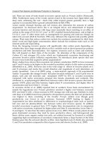
Fig. 2. SLAR geometry (after Mohr, 2005)

Active microwave RS observations usually employ a specific configuration: the side looking
aperture radar ( SLAR), whose line of sight (LOS) corresponds to a lateral view with respect
to the track direction (see Figure 2). First it introduces a projection factor in the range

resolution expression depending upon the incidence angle of the beam r =T·c/(2sin).
Secondly a SLAR image suffers from some distortions due to slant range configuration
resulting in errors related to the conversion of the measured slant range to the ground range;
this contributes to make the radar image very different from the optical view (Rosen et al.,
2000). When the surface is not flat, but we have topographic features, the terrain elevation
distorts the distance to the radar sensor in such a way that slopes facing the radar appear
shorter than they are when imaged in a normal map projection, while those that face away
from the radar appear longer than in the map the latter are illuminated by the radar sensor
very rarely: this is the foreshortening effect. Foreshortened areas appear brighter than their

surroundings because the reflected radar energy from the slope is compressed to correspond
to fewer pixels; when the slope of the terrain facing the radar is greater than the look-angle,
the top of the slope is closer to the radar than the bottom we have a layover; finally shadowing
can occur when terrain area cannot be illuminated and only system noise is imaged in the
shadowed areas of radar images (Curlander and McDonough, 1991). These errors are of
minor concern in observations where the slope area is imaged from below, that is to say in
Ground Based cases.

2.3 The azimuth or cross-range resolution and SAR
The energy transmitted by a conventional radar is concentrated into a beam with an angular
dimension, the field of view, 

,
basically determined by the ratio between the operating
wavelength and its mechanical size (Silver, 1986) and alike happens for the receiver which
collects the energy coming from the antenna beam. In a radar image targets that differ from
each other in their azimuth coordinates only, generate overlapping radar echoes and thus
they cannot be distinguished. Conceptually azimuth location can be achieved by changing
the viewing angle of a very directive antenna. In order to produce at a distance R a good
azimuth resolution, R 


, in the along-track direction, we need short ranges and large
antennas. At the same time to cover a wide swath, S, as requested e.g. in satellite geometry,
we need a large 

meaning a small antenna. Viewing a target during the entire time it is
within a beamwidth, determines a situation analogous to an artificially long antenna. If we
acquire the amplitude and phase of the echoes an artificially narrow beamwidth in terms of
resolution can be realized. The further a target is from the radar, the longer it is within the
actual beamwidth, the longer the “antenna” and hence the narrower the resolution
beamwidth. If the sensor is moving towards or away from the scattering object/surface, we
can measure the velocity of the scattering object by measuring the Doppler effect which
induces a frequency variation according to the apparent radial velocity of a certain scatterer
on the ground. In order to make use of the forward motion, both the amplitude and phase of
the return signal have to be recorded. The timing measurement is used to discriminate
individual cells across the satellite track while the Doppler-induced variations in the
frequency of the return signal are employed to provide the along track resolution. The SAR
platform flies along a straight trajectory with a constant velocity illuminating a strip of
terrain parallel to the flight track (see Figure 2). The data set can be stored in a two-
dimensional array according to the SAR imaging geometry. The first step in SAR processing
includes the pulse compression in range direction, usually denoted as range compression. The
range compression is followed by the azimuth compression, which also yields the principle
of the pulse compression technique. The azimuth chirp, which is approximately linear
frequency modulated, is determined by the wavelength, the forward velocity and the slant
range distance to the target. If all these parameters are known a priori, the reference function
for a certain slant range distance is calculated to obtain a desired geometrical resolution
after pulse compression in azimuth direction. A SAR image with a range independent
azimuth resolution is obtained (Curlander and McDonough, 1991). Finally the azimuth
compression is carried out. The final result of this acquisition and processing is a radar
image with fine spatial resolution both in range and in azimuth directions: a few meter

square cell from hundreds of kilometers.

GroundbasedSARinterferometry:anoveltoolforGeoscience 5


The backscattered signal has an extension in time T due to the pulse width and in order to
obtain a good range resolution we need a short pulse. However, recalling Fourier transform
properties, a short pulse width means a large frequency bandwidth. At the same time as
dictated by the radar equation, at large distances, high amplitude is requested as the pulse
energy determines the detection possibilities of the system i.e. its signal to noise ratio (S/N).
This means that in designing a radar we are faced with the problem to want a long pulse
with high energy and a wide bandwidth which implies a short pulse. To reduce these
difficulties a signal processing technique, namely pulse compression, obtained by using a
“chirp radar” (Ulaby et al., 1982) can be used. In this case the transmitted frequency is
varying linearly with time and by correlating the return signal with a frequency modulated
signal, a sharp peak is obtained for a distance related to the time offset. The resolution
depends on the ability to sample sufficiently often the returned signals not to be aliased by
the sampling rate.

Fig. 2. SLAR geometry (after Mohr, 2005)

Active microwave RS observations usually employ a specific configuration: the side looking
aperture radar ( SLAR), whose line of sight (LOS) corresponds to a lateral view with respect
to the track direction (see Figure 2). First it introduces a projection factor in the range
resolution expression depending upon the incidence angle of the beam r =T·c/(2sin).
Secondly a SLAR image suffers from some distortions due to slant range configuration
resulting in errors related to the conversion of the measured slant range to the ground range;
this contributes to make the radar image very different from the optical view (Rosen et al.,
2000). When the surface is not flat, but we have topographic features, the terrain elevation
distorts the distance to the radar sensor in such a way that slopes facing the radar appear

shorter than they are when imaged in a normal map projection, while those that face away
from the radar appear longer than in the map the latter are illuminated by the radar sensor
very rarely: this is the foreshortening effect. Foreshortened areas appear brighter than their

surroundings because the reflected radar energy from the slope is compressed to correspond
to fewer pixels; when the slope of the terrain facing the radar is greater than the look-angle,
the top of the slope is closer to the radar than the bottom we have a layover; finally shadowing
can occur when terrain area cannot be illuminated and only system noise is imaged in the
shadowed areas of radar images (Curlander and McDonough, 1991). These errors are of
minor concern in observations where the slope area is imaged from below, that is to say in
Ground Based cases.

2.3 The azimuth or cross-range resolution and SAR
The energy transmitted by a conventional radar is concentrated into a beam with an angular
dimension, the field of view, 

,
basically determined by the ratio between the operating
wavelength and its mechanical size (Silver, 1986) and alike happens for the receiver which
collects the energy coming from the antenna beam. In a radar image targets that differ from
each other in their azimuth coordinates only, generate overlapping radar echoes and thus
they cannot be distinguished. Conceptually azimuth location can be achieved by changing
the viewing angle of a very directive antenna. In order to produce at a distance R a good
azimuth resolution, R 

, in the along-track direction, we need short ranges and large
antennas. At the same time to cover a wide swath, S, as requested e.g. in satellite geometry,
we need a large 

meaning a small antenna. Viewing a target during the entire time it is

within a beamwidth, determines a situation analogous to an artificially long antenna. If we
acquire the amplitude and phase of the echoes an artificially narrow beamwidth in terms of
resolution can be realized. The further a target is from the radar, the longer it is within the
actual beamwidth, the longer the “antenna” and hence the narrower the resolution
beamwidth. If the sensor is moving towards or away from the scattering object/surface, we
can measure the velocity of the scattering object by measuring the Doppler effect which
induces a frequency variation according to the apparent radial velocity of a certain scatterer
on the ground. In order to make use of the forward motion, both the amplitude and phase of
the return signal have to be recorded. The timing measurement is used to discriminate
individual cells across the satellite track while the Doppler-induced variations in the
frequency of the return signal are employed to provide the along track resolution. The SAR
platform flies along a straight trajectory with a constant velocity illuminating a strip of
terrain parallel to the flight track (see Figure 2). The data set can be stored in a two-
dimensional array according to the SAR imaging geometry. The first step in SAR processing
includes the pulse compression in range direction, usually denoted as range compression. The
range compression is followed by the azimuth compression, which also yields the principle
of the pulse compression technique. The azimuth chirp, which is approximately linear
frequency modulated, is determined by the wavelength, the forward velocity and the slant
range distance to the target. If all these parameters are known a priori, the reference function
for a certain slant range distance is calculated to obtain a desired geometrical resolution
after pulse compression in azimuth direction. A SAR image with a range independent
azimuth resolution is obtained (Curlander and McDonough, 1991). Finally the azimuth
compression is carried out. The final result of this acquisition and processing is a radar
image with fine spatial resolution both in range and in azimuth directions: a few meter
square cell from hundreds of kilometers.

GeoscienceandRemoteSensing,NewAchievements6


3. SAR Interferometry from space


3.1Introduction
Interferometry is a technique which use the phase information retrieved from the interaction
of two different waves to retrieve temporal or spatial information on the waves propagation.
First developed in optics, during the 20
th
century it has been later applied to radio waves
and in the last decade to spaceborne SAR images. Since the SAR system is coherent, i.e.
transmits and receive a complex signal with high stability, it is possible to use its
interferometric signal, provided that propagation does not introduce decorrelation, namely
a loss of information in irreversible way. This means that the scattered signal of the two
images must be sufficiently correlated. We may combine images using different overpasses
(multi-pass interferometry) where a baseline, a path difference due to satellite track
separation, is present. In this case interferometric phase contains a contribution of
topography which can be taken into account through the use of a digital elevation model
(DEM). A simple scheme of how two images of the same area gathered from two slightly
different across track positions, interfere and produce phase fringes that can be used to
accurately determine the variation of the LOS distance is depicted in Figure 3. An
interferogram is the map whose pixel values, s
i
, are produced by conjugate multiplication of
every pixel of two complex SAR images I
1,i
, and I
2,i
in one image as shown in eq. 2a, where
I
1,i
and I
2,i

are the complex pixel amplitudes, R
1,i
and R
2,i
are the two slant range coordinates,
Bp,i is the baseline described by B
n
and B
p
, the baseline normal and parallel respectively to
the line of sight, the last the only component affecting the phase, noise,i is the phase noise
that is due to speckle and thermal noise and usually including contribution from scattering
too.


(2a)



(2b)

The amplitude of this product contains information on the noise of the phase observations
and it is related to coherence, discussed in the next paragraph. Starting from the phase in
equation (2b) and by assuming that the scene is stable, it is possible to derive a linear
expression for the variations of the interferogram phase, between different pixels (Ferretti J.,
2007; Askne J. et al., 2003):


(3)



Here Bn and R are defined above, is the difference in elevation angleR is the slant
range difference and z is the altitude difference between pixels in the interferogram. The
noise term is the phase noise, which determines how well the phase variations can be
determined, also quantified by the coherence as described below.


j
e
i
s
)
inoise,
Φ)
1i
R
2i
(R
λ
4π
j
e
*
i2,
I
i1,
I
*
i2,
I

i1,
I
i
s






















)
inoise,
Φ
pi

(B
λ
4π
j
e
*
i2,
I
i1,
I
i
s









2
sin
4
tan
4
4
 nz
R
B

R
R
B
B
noise
nn
n

The first term in (3) is purely a systematic effect that can easily be removed in the processing
by applying “the flat earth compensation". In the second term there is a direct relation
between the phase and the altitude in the image z. The last term represents the phase
ambiguity induced by the modulo 2 phase registration. The ambiguity has to be removed
in the processing by adding the correct integer number of 2 to each measured value. This is
called phase unwrapping. If the 2 ambiguities are removed this phase difference can be
used to calculate the off-nadir angle and the height variations i.e. a topographic map. As far
as the problem of phase unwrapping is concerned, this topic is not tackled with in this
chapter (see for instance Ghiglia & Romero, 1994). This factor can influence the choice of the
operating frequency: long wavelengths can represent a good compromise between a
moderate displacement sensitivity and a reduced occurrence of phase wrapping when the
expected landslide velocity is high.

Baseline cannot increase over certain limit where the coherence is lost (baseline
decorrelation effect). The use of the topographic effect which relates to the height of the
portion of terrain corresponding to a pixel in the interferogram is one of the successful
InSAR application, aiming at deriving a DEM of the imaged area (Zebker et al., 1986). It
disappears for image pairs taken exactly from the same position (zero baseline). In this
simpler case when further sources of phase variation are negligible the displacement of the
ith point is recovered from the interferometric phase, φ
i
by the following equation.



(4)

In GBInSAR this is the ordinary configuration which provides ‘‘topography-free’’
interferogram and whose phase can be directly related to terrain movements.
















Fig. 3. (Left) InSAR geometry. The along the track direction is perpendicular to the graph
plane. (Right) the rationale of the fringes formation due to baseline (Modified from Shang-
Ho, 2008).




4

i
i
r 
GroundbasedSARinterferometry:anoveltoolforGeoscience 7


3. SAR Interferometry from space

3.1Introduction
Interferometry is a technique which use the phase information retrieved from the interaction
of two different waves to retrieve temporal or spatial information on the waves propagation.
First developed in optics, during the 20
th
century it has been later applied to radio waves
and in the last decade to spaceborne SAR images. Since the SAR system is coherent, i.e.
transmits and receive a complex signal with high stability, it is possible to use its
interferometric signal, provided that propagation does not introduce decorrelation, namely
a loss of information in irreversible way. This means that the scattered signal of the two
images must be sufficiently correlated. We may combine images using different overpasses
(multi-pass interferometry) where a baseline, a path difference due to satellite track
separation, is present. In this case interferometric phase contains a contribution of
topography which can be taken into account through the use of a digital elevation model
(DEM). A simple scheme of how two images of the same area gathered from two slightly
different across track positions, interfere and produce phase fringes that can be used to
accurately determine the variation of the LOS distance is depicted in Figure 3. An
interferogram is the map whose pixel values, s
i
, are produced by conjugate multiplication of
every pixel of two complex SAR images I
1,i

, and I
2,i
in one image as shown in eq. 2a, where
I
1,i
and I
2,i
are the complex pixel amplitudes, R
1,i
and R
2,i
are the two slant range coordinates,
Bp,i is the baseline described by B
n
and B
p
, the baseline normal and parallel respectively to
the line of sight, the last the only component affecting the phase, noise,i is the phase noise
that is due to speckle and thermal noise and usually including contribution from scattering
too.


(2a)



(2b)

The amplitude of this product contains information on the noise of the phase observations
and it is related to coherence, discussed in the next paragraph. Starting from the phase in

equation (2b) and by assuming that the scene is stable, it is possible to derive a linear
expression for the variations of the interferogram phase, between different pixels (Ferretti J.,
2007; Askne J. et al., 2003):


(3)


Here Bn and R are defined above, is the difference in elevation angleR is the slant
range difference and z is the altitude difference between pixels in the interferogram. The
noise term is the phase noise, which determines how well the phase variations can be
determined, also quantified by the coherence as described below.


j
e
i
s
)
inoise,
Φ)
1i
R
2i
(R
λ
4π
j
e
*

i2,
I
i1,
I
*
i2,
I
i1,
I
i
s























)
inoise,
Φ
pi
(B
λ
4π
j
e
*
i2,
I
i1,
I
i
s









2
sin

4
tan
4
4
 nz
R
B
R
R
B
B
noise
nn
n

The first term in (3) is purely a systematic effect that can easily be removed in the processing
by applying “the flat earth compensation". In the second term there is a direct relation
between the phase and the altitude in the image z. The last term represents the phase
ambiguity induced by the modulo 2 phase registration. The ambiguity has to be removed
in the processing by adding the correct integer number of 2 to each measured value. This is
called phase unwrapping. If the 2 ambiguities are removed this phase difference can be
used to calculate the off-nadir angle and the height variations i.e. a topographic map. As far
as the problem of phase unwrapping is concerned, this topic is not tackled with in this
chapter (see for instance Ghiglia & Romero, 1994). This factor can influence the choice of the
operating frequency: long wavelengths can represent a good compromise between a
moderate displacement sensitivity and a reduced occurrence of phase wrapping when the
expected landslide velocity is high.

Baseline cannot increase over certain limit where the coherence is lost (baseline
decorrelation effect). The use of the topographic effect which relates to the height of the

portion of terrain corresponding to a pixel in the interferogram is one of the successful
InSAR application, aiming at deriving a DEM of the imaged area (Zebker et al., 1986). It
disappears for image pairs taken exactly from the same position (zero baseline). In this
simpler case when further sources of phase variation are negligible the displacement of the
ith point is recovered from the interferometric phase, φ
i
by the following equation.


(4)

In GBInSAR this is the ordinary configuration which provides ‘‘topography-free’’
interferogram and whose phase can be directly related to terrain movements.
















Fig. 3. (Left) InSAR geometry. The along the track direction is perpendicular to the graph

plane. (Right) the rationale of the fringes formation due to baseline (Modified from Shang-
Ho, 2008).




4
i
i
r 
GeoscienceandRemoteSensing,NewAchievements8


3.2 Coherence and phase
The statistical measurability of the interferometric phase from images collected at different
times is related to its coherence (Bamler and Just, 1993). The spatial distribution of this
parameter can be associated to the quality of the interferometric phase map. The
interferometric coherence is the amplitude of the correlation coefficient between the two
complex SAR images forming the interferogram. In a few words a common measure of the
degree of statistical similarity of two images can be calculated through the following
expression:

(5)


where c is coherence and the brackets < > mean the average value of the argument and  is
the corresponding interferometric phase, assuming the ensemble average can be determined
by spatial averaging. The assumption that dielectric characteristics are similar for both
acquisitions and have no impact on the interferometric phase cannot be assumed to have
general validity and deserves a specific analysis taking into account the relevant conditions

during each acquisition and in particular the time span between them (temporal baseline).
E.g. vegetated area are usually rapidly decorrelating. On the other hand some features as
buildings or artificial targets in coherence images may be stable over many years. Targets
with such performances are called "permanent scatterers ©" (see Ferretti et al. 2001) and by
using the phase of such reference points one may correct for the atmospheric screen effect
with specific algorithm (Colesanti et al., 2003). In general the measured phase difference can
be expressed as the summation of five different terms:

(6)

The first term 
base
is from baseline, 
topo
is due to topography, 
defor
is the ground
deformation term, 
atm
is due to atmospheric propagation and 
noise
resumes random
noise due different sources including the instrumental ones and variations occurring on the
phase of the scattering surfaces. Limiting factors are due to delays in the ionosphere and
atmosphere, satellite orbit stability variations occurred on the scattering surfaces during the
time elapsed between the two acquisitions (Zebker et al., 1992). Although we normally say
that microwaves are independent of clouds and atmospheric effects this is not entirely true
and troposphere, and sometimes ionosphere, can affect the phase delay of waves and the
accuracy of interferometric phase according to the water vapor and temperature
fluctuations. Lastly it must be remembered that errors introduced by coregistration of the

images can also affect coherence. The advantage of a ground based approach is mainly due
to two factors: its zero baseline condition and its elevate temporal sampling both deeply
reducing the decorrelation sources.

4. Ground Based SAR interferometry

4.1 The landing of a space technique
It is possible to acquire SAR images through a portable SAR to be installed in stable area.
The motion for synthesizing the SAR image is obtained through a linear rail where a
microwave transceiver moves regularly. Ground-based radar installations are usually at
noiseatmdefortopobase




















j
ce
IIII
II




2211
*
21

their best when monitoring small scale phenomena like buildings, small urban area or single
hillsides, while imaging from satellite radar is able to monitor a very large area. As for
satellite cases GBSAR radar images acquired at different dates can be fruitful for
interferometry when the decorrelation among different images is maintained low. In ground
based observations with respect to satellite sensors there is the necessity of finding a site
with good visibility and from where the component of the displacement along the LOS is the
major part. Recent papers have been issued about the feasibility of airborne (Reigber et al.,
2003), or Ground Based radar interferometry based on portable instrumentation as a tool for
monitoring buildings or structures (Tarchi et al. 1997), landslides (Tarchi et al., 2003b), (Leva
et al. 2003), glaciers (Luzi et al. 2007). On the other hand satellite observations are sometimes
not fully satisfactory because of a lengthy repeat pass time or of changes on observational
geometry. Satellite, airborne and ground based radar interferometry are derived from the
same physical principles but they are often characterized by specific problems mainly due to
the difference of the geometry of the observation. A number of experimental results
demonstrated the GBSAR effectiveness for remote monitoring of terrain slopes and as an
early warning system to assess the risk of rapid landslides: here we briefly recall three
examples taken from recent literature. The first is the monitoring of a slope where a large
landslide is located. The second deals with an instable slope in a volcanic area where

alerting procedures are a must. Finally an example of a research devoted to the
interpretation of interferometric data collected through a GB SAR system to retrieve the
characteristics of a snow cover is discussed.

4.2 The GB DInSAR instrumentation
Despite the use of the same physical principle, the satellite and ground based approaches
differ in some aspects. In particular radar sensors of different kinds are usually employed
mainly because of technical and operational reasons. While satellite SAR systems due to the
need of a fast acquisition are based on standard pulse radar, continuous wave step
frequency (CWSF) radar are usually preferred in ground based observations. The Joint
Research Center (JRC) has been a pioneer of this technology and here the first prototype was
born. The first paper about a GB SAR interferometry experiment dates back to 1999 (Tarchi
et al., 1999), reporting a demonstration test on dam financed by the EC JRC in Ispra and the
used equipment was composed of a radar sensor based on Vectorial Network Analyser
(VNA), a coherent transmitting and receiving set-up, a mechanical guide, a PC based data
acquisition and a control unit.

After some years a specific system, known as GBInSAR LiSA, reached an operative state and
became available to the market by Ellegi-LiSALab company which on June 2003 obtained an
exclusive licence to commercially exploit this technology from JRC. The use of VNA to
realize a scatterometer, i.e. a coherent calibrated radar for RCS measurement, has been
frequently used by researchers (e.g. Strozzi et al., 1998) as it easily makes a powerful tool for
coherent radar measurements available. The basic and simplest schematic of the
radiofrequency set-up used for radar measurements is shown in Figure 4 together with a
simple scheme of the GBSAR acquisition. Advanced versions of this set-up have been
realized in the next years to improve stability and frequency capabilities (Rudolf et al., 1999
and Noferini et al., 2005). This apparatus is able to generate microwave signals at definite
increasing frequencies sweeping a radiofrequency band. This approach apparently different
GroundbasedSARinterferometry:anoveltoolforGeoscience 9



3.2 Coherence and phase
The statistical measurability of the interferometric phase from images collected at different
times is related to its coherence (Bamler and Just, 1993). The spatial distribution of this
parameter can be associated to the quality of the interferometric phase map. The
interferometric coherence is the amplitude of the correlation coefficient between the two
complex SAR images forming the interferogram. In a few words a common measure of the
degree of statistical similarity of two images can be calculated through the following
expression:

(5)


where c is coherence and the brackets < > mean the average value of the argument and  is
the corresponding interferometric phase, assuming the ensemble average can be determined
by spatial averaging. The assumption that dielectric characteristics are similar for both
acquisitions and have no impact on the interferometric phase cannot be assumed to have
general validity and deserves a specific analysis taking into account the relevant conditions
during each acquisition and in particular the time span between them (temporal baseline).
E.g. vegetated area are usually rapidly decorrelating. On the other hand some features as
buildings or artificial targets in coherence images may be stable over many years. Targets
with such performances are called "permanent scatterers ©" (see Ferretti et al. 2001) and by
using the phase of such reference points one may correct for the atmospheric screen effect
with specific algorithm (Colesanti et al., 2003). In general the measured phase difference can
be expressed as the summation of five different terms:

(6)

The first term 
base

is from baseline, 
topo
is due to topography, 
defor
is the ground
deformation term, 
atm
is due to atmospheric propagation and 
noise
resumes random
noise due different sources including the instrumental ones and variations occurring on the
phase of the scattering surfaces. Limiting factors are due to delays in the ionosphere and
atmosphere, satellite orbit stability variations occurred on the scattering surfaces during the
time elapsed between the two acquisitions (Zebker et al., 1992). Although we normally say
that microwaves are independent of clouds and atmospheric effects this is not entirely true
and troposphere, and sometimes ionosphere, can affect the phase delay of waves and the
accuracy of interferometric phase according to the water vapor and temperature
fluctuations. Lastly it must be remembered that errors introduced by coregistration of the
images can also affect coherence. The advantage of a ground based approach is mainly due
to two factors: its zero baseline condition and its elevate temporal sampling both deeply
reducing the decorrelation sources.

4. Ground Based SAR interferometry

4.1 The landing of a space technique
It is possible to acquire SAR images through a portable SAR to be installed in stable area.
The motion for synthesizing the SAR image is obtained through a linear rail where a
microwave transceiver moves regularly. Ground-based radar installations are usually at
noiseatmdefortopobase




















j
ce
IIII
II




2211
*
21


their best when monitoring small scale phenomena like buildings, small urban area or single
hillsides, while imaging from satellite radar is able to monitor a very large area. As for
satellite cases GBSAR radar images acquired at different dates can be fruitful for
interferometry when the decorrelation among different images is maintained low. In ground
based observations with respect to satellite sensors there is the necessity of finding a site
with good visibility and from where the component of the displacement along the LOS is the
major part. Recent papers have been issued about the feasibility of airborne (Reigber et al.,
2003), or Ground Based radar interferometry based on portable instrumentation as a tool for
monitoring buildings or structures (Tarchi et al. 1997), landslides (Tarchi et al., 2003b), (Leva
et al. 2003), glaciers (Luzi et al. 2007). On the other hand satellite observations are sometimes
not fully satisfactory because of a lengthy repeat pass time or of changes on observational
geometry. Satellite, airborne and ground based radar interferometry are derived from the
same physical principles but they are often characterized by specific problems mainly due to
the difference of the geometry of the observation. A number of experimental results
demonstrated the GBSAR effectiveness for remote monitoring of terrain slopes and as an
early warning system to assess the risk of rapid landslides: here we briefly recall three
examples taken from recent literature. The first is the monitoring of a slope where a large
landslide is located. The second deals with an instable slope in a volcanic area where
alerting procedures are a must. Finally an example of a research devoted to the
interpretation of interferometric data collected through a GB SAR system to retrieve the
characteristics of a snow cover is discussed.

4.2 The GB DInSAR instrumentation
Despite the use of the same physical principle, the satellite and ground based approaches
differ in some aspects. In particular radar sensors of different kinds are usually employed
mainly because of technical and operational reasons. While satellite SAR systems due to the
need of a fast acquisition are based on standard pulse radar, continuous wave step
frequency (CWSF) radar are usually preferred in ground based observations. The Joint
Research Center (JRC) has been a pioneer of this technology and here the first prototype was
born. The first paper about a GB SAR interferometry experiment dates back to 1999 (Tarchi

et al., 1999), reporting a demonstration test on dam financed by the EC JRC in Ispra and the
used equipment was composed of a radar sensor based on Vectorial Network Analyser
(VNA), a coherent transmitting and receiving set-up, a mechanical guide, a PC based data
acquisition and a control unit.

After some years a specific system, known as GBInSAR LiSA, reached an operative state and
became available to the market by Ellegi-LiSALab company which on June 2003 obtained an
exclusive licence to commercially exploit this technology from JRC. The use of VNA to
realize a scatterometer, i.e. a coherent calibrated radar for RCS measurement, has been
frequently used by researchers (e.g. Strozzi et al., 1998) as it easily makes a powerful tool for
coherent radar measurements available. The basic and simplest schematic of the
radiofrequency set-up used for radar measurements is shown in Figure 4 together with a
simple scheme of the GBSAR acquisition. Advanced versions of this set-up have been
realized in the next years to improve stability and frequency capabilities (Rudolf et al., 1999
and Noferini et al., 2005). This apparatus is able to generate microwave signals at definite
increasing frequencies sweeping a radiofrequency band. This approach apparently different
GeoscienceandRemoteSensing,NewAchievements10


from that of the standard pulse radar owns the same physical meaning because a temporal
pulse can be obtained after Fourier anti transforming the frequency data (the so called
synthetic pulse approach).

The rapid grow of microwave technology occurred in the last years encouraged the
development and realization of different instruments (Pipia et al., 2007 Bernardini et al.,
2007); recently a ground based interferometer with a non-SAR approach has been designed
with similar monitoring purposes (Werner et al., 2008). Data are processed in real time by
means of a SAR processor. An algorithm combines the received amplitude and phase values
stored for each position and frequency values, to return complex amplitudes (Fortuny J. and
A.J. Sieber, 1994). The optimization of focusing algorithms has been recently updated by

Reale et al, 2008; Fortuny, 2009. To reduce the effect of side lobes in range and azimuth
synthesis (Mensa D.L. , 1991) , data are corrected by means of a window functions (Kaiser,
Hamming etc), for range and azimuth synthesis. The attainable spatial resolutions and
ambiguities are related to radar parameters through the relationships shown in Table 1. The
accuracy of the measured phase is usually a fraction of the operated wavelength: by using
centimetre wavelengths millimetre accuracy can be attained. As previously introduced, the
phase from complex images can suffer from the ambiguity due to the impossibility of
distinguishing between phases that differ by 2. Single radar images are affected by noise
and related interferometric maps must be obtained through an adequate phase stability
between the pair of images: only pairs whose coherence loss can not affect the accuracy of
the interferometric maps are usable. This task is of major difficulty when the considered
time period is of the order of months.













Fig. 4. A) Basic scheme of the RF section of the C band transceiver based on the Vectorial
Network Analyser VNA. B) GB SAR acquisition through a linear motion.

A detailed analysis to the possible causes of decorrelation in the specific case of GBInSAR
observations gathering many images per day for continuous measurements has been

discussed by some researchers (Luzi et al., 2004 and Pipia et al. ,2007) while for campaigns
carried out on landslides moving only few centimeters per year, when the sensor is
periodically installed at repeated intervals several months apart over the observation period,
a novel method has been proposed (Noferini et al. 2005).


Range resolution

B
c
Rr
2


Azimuth resolution

R
L
Raz
x
c

2


Non ambiguous range (m )

f
c
R

na


2

Table 1. calculated resolution available from a CWSF radar observation; B radiofrequency
bandwidth, 
c
in vacuum wavelength, f frequency step, Lx rail length, R range, c light
velocity.

5. Examples of GB INSAR data collections

5.1. The monitoring of a landslide
This first example of how to benefit from the use of GBInSAR in Geoscience, is its employ as
a monitoring tool for instable slopes, a well consolidated application largely reported in
literature (Leva et al. 2003, Pieraccini et al., 2003, Tarchi et al., 2003a). The investigation and
interpretation of the patterns of movement associated with landslides have been undertaken
by using a wide range of techniques, including the use of survey markers: extensometers,
inclinometers, analogue and digital photogrammetry, both terrestrial and aerial. In general,
they suffer from serious shortcomings in terms of spatial resolution. GB SAR, thanks to its
spatial and temporal sampling can overcome the restrictions of the conventional point-wise
measurement. Here some results of an experimental campaign carried out through a
portable GB radar to survey a large active landslide, the “Tessina landslide”, near Belluno in
north-eastern Italy are shown. In this site a exhaustive conventional networks of sensors
fundamental to validate the proposed technique were at our disposal. For the same reason
this site has been used by different research teams to test their instrumentation, starting
since the first campaign carried out by JRC in 2000 (Tarchi et al., 2003a), following with
University of Florence in Luzi et al. 2006 and later with Bernardini et al., 2007 and Werner et
al., 2008. The GBInSAR monitoring executes analyzing maps of phase differences or

equivalently displacements’ map of the observed scenario, obtained from time sequences of
SAR images.

5.2 The test site
The area affected by the landslide extends from an elevation of 1200 m a.s.l at the crown
down to 610 m a.s.l. at the toe of the mudflow . Its total track length is approximately 3 Km,
and its maximum width is about 500 m, in the rear scar area, with a maximum depth of
about 50 m. Range measurements in different points were carried out through conventional
instrumentation with benchmarks positioned in different locations as depicted in Figure 5,
where a sight from the measurements facility is shown. Two of the optical control points
correspond to high reflecting radar targets. In particular, point 1 refers to a passive corner
reflector (PCR), an artificial target usually used as calibrator, which consists of a metal
trihedral with a size of 50. cm. Point 2 is an active radar calibrator (ARC), specifically
designed and built for this experimentation: an amplifier of the radar signal which allows
acquisition of high reflection pixels on the radar image at far distances that are useful for
amplitude calibration (radiometric calibration) and map geo-referencing. The GB radar
instrumentation available for the experiments here reported consists of a microwave (C
band) transceiver unit based on the HP8753D VNA, a linear horizontal rail where the
GroundbasedSARinterferometry:anoveltoolforGeoscience 11


from that of the standard pulse radar owns the same physical meaning because a temporal
pulse can be obtained after Fourier anti transforming the frequency data (the so called
synthetic pulse approach).

The rapid grow of microwave technology occurred in the last years encouraged the
development and realization of different instruments (Pipia et al., 2007 Bernardini et al.,
2007); recently a ground based interferometer with a non-SAR approach has been designed
with similar monitoring purposes (Werner et al., 2008). Data are processed in real time by
means of a SAR processor. An algorithm combines the received amplitude and phase values

stored for each position and frequency values, to return complex amplitudes (Fortuny J. and
A.J. Sieber, 1994). The optimization of focusing algorithms has been recently updated by
Reale et al, 2008; Fortuny, 2009. To reduce the effect of side lobes in range and azimuth
synthesis (Mensa D.L. , 1991) , data are corrected by means of a window functions (Kaiser,
Hamming etc), for range and azimuth synthesis. The attainable spatial resolutions and
ambiguities are related to radar parameters through the relationships shown in Table 1. The
accuracy of the measured phase is usually a fraction of the operated wavelength: by using
centimetre wavelengths millimetre accuracy can be attained. As previously introduced, the
phase from complex images can suffer from the ambiguity due to the impossibility of
distinguishing between phases that differ by 2. Single radar images are affected by noise
and related interferometric maps must be obtained through an adequate phase stability
between the pair of images: only pairs whose coherence loss can not affect the accuracy of
the interferometric maps are usable. This task is of major difficulty when the considered
time period is of the order of months.













Fig. 4. A) Basic scheme of the RF section of the C band transceiver based on the Vectorial
Network Analyser VNA. B) GB SAR acquisition through a linear motion.


A detailed analysis to the possible causes of decorrelation in the specific case of GBInSAR
observations gathering many images per day for continuous measurements has been
discussed by some researchers (Luzi et al., 2004 and Pipia et al. ,2007) while for campaigns
carried out on landslides moving only few centimeters per year, when the sensor is
periodically installed at repeated intervals several months apart over the observation period,
a novel method has been proposed (Noferini et al. 2005).


Range resolution
B
c
Rr
2


Azimuth resolution

R
L
Raz
x
c

2


Non ambiguous range (m )

f
c

R
na


2

Table 1. calculated resolution available from a CWSF radar observation; B radiofrequency
bandwidth, 
c
in vacuum wavelength, f frequency step, Lx rail length, R range, c light
velocity.

5. Examples of GB INSAR data collections

5.1. The monitoring of a landslide
This first example of how to benefit from the use of GBInSAR in Geoscience, is its employ as
a monitoring tool for instable slopes, a well consolidated application largely reported in
literature (Leva et al. 2003, Pieraccini et al., 2003, Tarchi et al., 2003a). The investigation and
interpretation of the patterns of movement associated with landslides have been undertaken
by using a wide range of techniques, including the use of survey markers: extensometers,
inclinometers, analogue and digital photogrammetry, both terrestrial and aerial. In general,
they suffer from serious shortcomings in terms of spatial resolution. GB SAR, thanks to its
spatial and temporal sampling can overcome the restrictions of the conventional point-wise
measurement. Here some results of an experimental campaign carried out through a
portable GB radar to survey a large active landslide, the “Tessina landslide”, near Belluno in
north-eastern Italy are shown. In this site a exhaustive conventional networks of sensors
fundamental to validate the proposed technique were at our disposal. For the same reason
this site has been used by different research teams to test their instrumentation, starting
since the first campaign carried out by JRC in 2000 (Tarchi et al., 2003a), following with
University of Florence in Luzi et al. 2006 and later with Bernardini et al., 2007 and Werner et

al., 2008. The GBInSAR monitoring executes analyzing maps of phase differences or
equivalently displacements’ map of the observed scenario, obtained from time sequences of
SAR images.

5.2 The test site
The area affected by the landslide extends from an elevation of 1200 m a.s.l at the crown
down to 610 m a.s.l. at the toe of the mudflow . Its total track length is approximately 3 Km,
and its maximum width is about 500 m, in the rear scar area, with a maximum depth of
about 50 m. Range measurements in different points were carried out through conventional
instrumentation with benchmarks positioned in different locations as depicted in Figure 5,
where a sight from the measurements facility is shown. Two of the optical control points
correspond to high reflecting radar targets. In particular, point 1 refers to a passive corner
reflector (PCR), an artificial target usually used as calibrator, which consists of a metal
trihedral with a size of 50. cm. Point 2 is an active radar calibrator (ARC), specifically
designed and built for this experimentation: an amplifier of the radar signal which allows
acquisition of high reflection pixels on the radar image at far distances that are useful for
amplitude calibration (radiometric calibration) and map geo-referencing. The GB radar
instrumentation available for the experiments here reported consists of a microwave (C
band) transceiver unit based on the HP8753D VNA, a linear horizontal rail where the
GeoscienceandRemoteSensing,NewAchievements12


antennas move while scanning the synthetic aperture, and a PC controlling the VNA, the
antenna motion, the data recording, and all the other operations needed to carry out the
measurement. Collected radar images are used for the calculation of the interferogram and
converted into multi-temporal maps of the displacement component along the radar line of
sight in geo-referenced raster format for GIS applications.

The measurement campaign on the Tessina landslide was continuously carried out between
the 4th of June and the 9th of June 2004. The instrumentation was installed at an elevation of

997.3 m a.s.l., in a stable area on the opposite slope in front of the landslide, mainly visible at
a minimum and maximum distance of 100. m and 500. m, respectively. The mechanical
frame was fixed on a concrete wall. The radar image exhibits a fixed spatial resolution of 2 m
along the range direction and a variable cross-range spatial resolution better than 6 m. The
area selected for SAR imaging is a rectangle with size 400m per 1000m. The images obtained
with the ground-based SAR system are usually projected as a two dimensional image of the
scenario along two directions, range and azimuth, with a plane representation.

Fig. 5. View from the radar installation of the monitored area. Red figures indicate
benchmarks for optical measuring (After Luzi et al., 2006).

The interpretation of bi-dimensional SAR images of a complex scenario, where terrain slope
changes abruptly, is often unsatisfactory for comparison to an optical view. The availability
of a DEM of the observed scene allows us to obtain SAR images on a three-dimensional
space where radar and optical features are better detectable. Figure 6 shows an example of
an intensity SAR image projected on the DEM: all three coordinates of the pixel are
reconstructed. In this image the position of the radar is marked by a red dot; the signatures
of the two high reflectivity targets, consisting of the passive corner reflector (PCR) and the
active radar calibrator (ACR), used for referencing the map, are neat.

5.3 Data analysis
As previously discussed in GB SAR observations the main source of decorrelation is that one
due to atmospheric propagation. At the C band radar frequencies the attenuation due to
atmospheric path is low but the signal propagating through atmosphere suffers anyhow a
time delay, mainly changing with air humidity and temperature fluctuations which ask for
correction procedures of the acquired data. Briefly, the applied method consists of
subtracting the phase value measured on a stable, highly reflecting reference point artificial

or natural, from the measured phase of the selected pixel. In our case the characteristics of
the observed scenario, mainly composed of sliding bare soil or by sparse vegetation, made it

difficult to find stable natural scatterers. The passive corner reflector and the active radar
calibrator were installed in two different positions along the upper contour of the landslide,
and their positions were continuously checked by means of a theodolite to verify their
effective stability. The PCR position, measured by theodolite, resulted stable along the entire
duration of the campaign within +-1mm. The scarce vegetation on the main area under
investigation allowed to get high coherence values.


Fig. 6. Radar intensity image (arbitrary units) of the monitored slope obtained with data
collected on 6 June 2004 and rendered on Digital Elevation Model of the slope. Two high
reflectivity targets, the passive corn reflector (PCR) and the active calibrator (ARC) are
indicated (After Luzi et al., 2006).

Displacements measured by the theodolite and corresponding values retrieved from radar
data are plotted as a function of time in Figure 7. Some data gaps are due to interruptions
during heavy rain events or small adjustments on the installation of radar targets. The
measured phase of point 1 (PCR), whose position was confirmed to be stable within the
millimetric accuracy of the optical instrumentation, is subtracted from the measured phases
of the other points to take into account atmospheric induced error. Observing Figure 7,
agreement appears viable and the displacements measured respectively through optical
benchmarks and radar show similar trends. A noticeable discrepancy appears for the faster
points (P10 and P17), whose corresponding pixels include inhomogeneous areas in terms of
slope and surface characteristics. The uncertainty can be ascribed to the fact that the
theodolite measures a single point, while radar data are obtained through a spatial
averaging on an area of some meters. From these data a maximum 2.5mm/30’ displacement
rate results. Regarding phase wrapping, this rate value ensures that the phase variation
occurred between two subsequent measurements (< 30’) is small compared to the centimetre
half-wavelength.
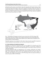
Moving from a point-wise analysis to the entire observed surface, the displacement of each
pixel can be depicted in colour scale corresponding to different values in millimetres,

making it possible to compare the radar data with an overlapped map of the scenario. In
Figure 8 is shown the interferometric map obtained through a masking procedure which
excludes areas with coherence lower than the 0.7 threshold. The geometry of observation
GroundbasedSARinterferometry:anoveltoolforGeoscience 13


antennas move while scanning the synthetic aperture, and a PC controlling the VNA, the
antenna motion, the data recording, and all the other operations needed to carry out the
measurement. Collected radar images are used for the calculation of the interferogram and
converted into multi-temporal maps of the displacement component along the radar line of
sight in geo-referenced raster format for GIS applications.

The measurement campaign on the Tessina landslide was continuously carried out between
the 4th of June and the 9th of June 2004. The instrumentation was installed at an elevation of
997.3 m a.s.l., in a stable area on the opposite slope in front of the landslide, mainly visible at
a minimum and maximum distance of 100. m and 500. m, respectively. The mechanical
frame was fixed on a concrete wall. The radar image exhibits a fixed spatial resolution of 2 m
along the range direction and a variable cross-range spatial resolution better than 6 m. The
area selected for SAR imaging is a rectangle with size 400m per 1000m. The images obtained
with the ground-based SAR system are usually projected as a two dimensional image of the
scenario along two directions, range and azimuth, with a plane representation.

Fig. 5. View from the radar installation of the monitored area. Red figures indicate
benchmarks for optical measuring (After Luzi et al., 2006).

The interpretation of bi-dimensional SAR images of a complex scenario, where terrain slope
changes abruptly, is often unsatisfactory for comparison to an optical view. The availability
of a DEM of the observed scene allows us to obtain SAR images on a three-dimensional
space where radar and optical features are better detectable. Figure 6 shows an example of
an intensity SAR image projected on the DEM: all three coordinates of the pixel are

reconstructed. In this image the position of the radar is marked by a red dot; the signatures
of the two high reflectivity targets, consisting of the passive corner reflector (PCR) and the
active radar calibrator (ACR), used for referencing the map, are neat.

5.3 Data analysis
As previously discussed in GB SAR observations the main source of decorrelation is that one
due to atmospheric propagation. At the C band radar frequencies the attenuation due to
atmospheric path is low but the signal propagating through atmosphere suffers anyhow a
time delay, mainly changing with air humidity and temperature fluctuations which ask for
correction procedures of the acquired data. Briefly, the applied method consists of
subtracting the phase value measured on a stable, highly reflecting reference point artificial

or natural, from the measured phase of the selected pixel. In our case the characteristics of
the observed scenario, mainly composed of sliding bare soil or by sparse vegetation, made it
difficult to find stable natural scatterers. The passive corner reflector and the active radar
calibrator were installed in two different positions along the upper contour of the landslide,
and their positions were continuously checked by means of a theodolite to verify their
effective stability. The PCR position, measured by theodolite, resulted stable along the entire
duration of the campaign within +-1mm. The scarce vegetation on the main area under
investigation allowed to get high coherence values.


Fig. 6. Radar intensity image (arbitrary units) of the monitored slope obtained with data
collected on 6 June 2004 and rendered on Digital Elevation Model of the slope. Two high
reflectivity targets, the passive corn reflector (PCR) and the active calibrator (ARC) are
indicated (After Luzi et al., 2006).

Displacements measured by the theodolite and corresponding values retrieved from radar
data are plotted as a function of time in Figure 7. Some data gaps are due to interruptions
during heavy rain events or small adjustments on the installation of radar targets. The

measured phase of point 1 (PCR), whose position was confirmed to be stable within the
millimetric accuracy of the optical instrumentation, is subtracted from the measured phases
of the other points to take into account atmospheric induced error. Observing Figure 7,
agreement appears viable and the displacements measured respectively through optical
benchmarks and radar show similar trends. A noticeable discrepancy appears for the faster
points (P10 and P17), whose corresponding pixels include inhomogeneous areas in terms of
slope and surface characteristics. The uncertainty can be ascribed to the fact that the
theodolite measures a single point, while radar data are obtained through a spatial
averaging on an area of some meters. From these data a maximum 2.5mm/30’ displacement
rate results. Regarding phase wrapping, this rate value ensures that the phase variation
occurred between two subsequent measurements (< 30’) is small compared to the centimetre
half-wavelength.
Moving from a point-wise analysis to the entire observed surface, the displacement of each
pixel can be depicted in colour scale corresponding to different values in millimetres,
making it possible to compare the radar data with an overlapped map of the scenario. In
Figure 8 is shown the interferometric map obtained through a masking procedure which
excludes areas with coherence lower than the 0.7 threshold. The geometry of observation
GeoscienceandRemoteSensing,NewAchievements14


was never changed during the overall campaign, and approximately 300 images were
collected, one every 16-18 minutes. The map in Figure 8 is obtained considering the data
collected from 17h.48m GMT+1 to 22h.53m GMT+1 of the 6 June. As mentioned above, these
data are very interesting because they refer to areas that are inaccessible for the placement of
benchmarks. For example, we can monitor a minor central area where the movement rate is
so high as to cause displacement of up to ten centimetres in 5 hours, while the rest of the
landslide area shows a slower motion, about 1mm/hour. This map making available an
estimate of the displacement along the LoS over the entire slope, can be the starting point to
understand and analyze the behaviour of the landslide. Relationships between slope
movement and other factors as rain rate, can be studied (Luzi et al., 2006) to understand

landslide dynamic.

Fig. 7. Displacements measured by the theodolite (solid line) and corresponding values
retrieved from radar data (symbols) for some reference points supplied with optical
benchmarks, as a function of time. Figure points refers to Figure 5. (After Luzi et al., 2006)


Fig. 8. Displacement map projected on the corresponding cartographic map obtained with
data from 17:48 to 22:53 of 6 June. Colour bar represents displacement towards radar
location (approaching), in mm (After Luzi et al., 2006).



5.4 Volcano deformations monitoring through GBInSAR monitoring

5.4.1 Introduction
Deformations monitoring through GB SAR has been applied in several different
circumstances of slope instability. One of the most interesting case is the monitoring of a
Volcanic area, presently in progress, and herein briefly described. When non-remote
conventional approach can be inapplicable GB SAR can offer a good opportunity. To
continuously monitor the behaviour of the morphological depression, known as Sciara del
Fuoco, SdF, with alerting purposes, a GB-In SAR system, working at Ku band, was set up on
the stable right flank of the Stromboli volcano in Italy. The monitoring started in March 2003
(Antonello et al., 2003) and ever since it is continuously acquiring. This lateral location was
chosen due to the logistic impossibility to place the system in front of the unstable slope and
permitted to follow the temporal and spatial evolution of the mass movement in the SdF
and to obtain information about the crater area through interferometric maps acquired with
ten minutes cadence. This monitoring was arranged as a consequence of the collapse of a
large landslide which caused a tsunami on December 2002. More generally the presence of
deformations in a volcanic area can be often related to volcanic activities. Stromboli volcano

is characterized by a typical “Strombolian activity” which consists of very low energy
explosions, every 10-15 minutes. The investigation and interpretation of the movement
associated with deformations have been undertaken by using a wide range of techniques,
including the use of survey markers, extensometers, inclinometers. However, they often
incur serious shortcomings in terms of spatial or temporal resolutions. Although these
techniques provide abundant datasets on movement styles, they are difficult to interpret in
terms of the overall evolution of movement and cannot be installed in a risky area as the
slope of an active volcano. GBDInSAR, can provide excellent spatial coverage and temporal
resolution, and large movement events can be easily captured from remote.

5.4.2 The test site and the experimental data
The GB SAR installed in Stromboli Island, was designed by the Joint Research Centre of the
European Commission (Rudolf & Tarchi, 1999) and it is built and supplied by Ellegi/Lisalab
company. Data are acquired from an elevation of 400 m a.s.l. and at an average distance
from the target area of about 600 m. The instrument points up toward the NE Crater, with a
25° inclination angle of the radar antennas. It is continuously active since 20 February 2003
(Antonello et al., 2003; Antonello et al., 2007) and produces, on average, 120 images per day
of the area under investigation (NE flank of crater and the upper part of the SdF). With an
accuracy of the measurement of less than 1 mm it produces a synthesized radar image of the
observed area every 12 minutes, with a pixel resolution of about 2 m in range, and 2 m on
average in cross range. The interferometric analysis of sequences of consecutive images
allows us to derive the entire displacement field of the observed portion of the SdF and of
the crater along the LoS in the time interval. A negative displacement means a shortening of
the LoS length. On the crater area this direction of movement corresponds to the inflation of
the volcanic cone while, on the SdF, this is usually related to a local bulging or to the
downslope sliding of the volcanoclastic material accumulated on the SdF slope.
Conversely, a positive value of displacement identifies a movement backward with respect
to the sensor that on the crater area could be related to the deflation of the volcanic cone. As
usual the radar image must be interpreted after a carefully understanding of the monitored
GroundbasedSARinterferometry:anoveltoolforGeoscience 15



was never changed during the overall campaign, and approximately 300 images were
collected, one every 16-18 minutes. The map in Figure 8 is obtained considering the data
collected from 17h.48m GMT+1 to 22h.53m GMT+1 of the 6 June. As mentioned above, these
data are very interesting because they refer to areas that are inaccessible for the placement of
benchmarks. For example, we can monitor a minor central area where the movement rate is
so high as to cause displacement of up to ten centimetres in 5 hours, while the rest of the
landslide area shows a slower motion, about 1mm/hour. This map making available an
estimate of the displacement along the LoS over the entire slope, can be the starting point to
understand and analyze the behaviour of the landslide. Relationships between slope
movement and other factors as rain rate, can be studied (Luzi et al., 2006) to understand
landslide dynamic.

Fig. 7. Displacements measured by the theodolite (solid line) and corresponding values
retrieved from radar data (symbols) for some reference points supplied with optical
benchmarks, as a function of time. Figure points refers to Figure 5. (After Luzi et al., 2006)


Fig. 8. Displacement map projected on the corresponding cartographic map obtained with
data from 17:48 to 22:53 of 6 June. Colour bar represents displacement towards radar
location (approaching), in mm (After Luzi et al., 2006).



5.4 Volcano deformations monitoring through GBInSAR monitoring

5.4.1 Introduction
Deformations monitoring through GB SAR has been applied in several different
circumstances of slope instability. One of the most interesting case is the monitoring of a

Volcanic area, presently in progress, and herein briefly described. When non-remote
conventional approach can be inapplicable GB SAR can offer a good opportunity. To
continuously monitor the behaviour of the morphological depression, known as Sciara del
Fuoco, SdF, with alerting purposes, a GB-In SAR system, working at Ku band, was set up on
the stable right flank of the Stromboli volcano in Italy. The monitoring started in March 2003
(Antonello et al., 2003) and ever since it is continuously acquiring. This lateral location was
chosen due to the logistic impossibility to place the system in front of the unstable slope and
permitted to follow the temporal and spatial evolution of the mass movement in the SdF
and to obtain information about the crater area through interferometric maps acquired with
ten minutes cadence. This monitoring was arranged as a consequence of the collapse of a
large landslide which caused a tsunami on December 2002. More generally the presence of
deformations in a volcanic area can be often related to volcanic activities. Stromboli volcano
is characterized by a typical “Strombolian activity” which consists of very low energy
explosions, every 10-15 minutes. The investigation and interpretation of the movement
associated with deformations have been undertaken by using a wide range of techniques,
including the use of survey markers, extensometers, inclinometers. However, they often
incur serious shortcomings in terms of spatial or temporal resolutions. Although these
techniques provide abundant datasets on movement styles, they are difficult to interpret in
terms of the overall evolution of movement and cannot be installed in a risky area as the
slope of an active volcano. GBDInSAR, can provide excellent spatial coverage and temporal
resolution, and large movement events can be easily captured from remote.

5.4.2 The test site and the experimental data
The GB SAR installed in Stromboli Island, was designed by the Joint Research Centre of the
European Commission (Rudolf & Tarchi, 1999) and it is built and supplied by Ellegi/Lisalab
company. Data are acquired from an elevation of 400 m a.s.l. and at an average distance
from the target area of about 600 m. The instrument points up toward the NE Crater, with a
25° inclination angle of the radar antennas. It is continuously active since 20 February 2003
(Antonello et al., 2003; Antonello et al., 2007) and produces, on average, 120 images per day
of the area under investigation (NE flank of crater and the upper part of the SdF). With an

accuracy of the measurement of less than 1 mm it produces a synthesized radar image of the
observed area every 12 minutes, with a pixel resolution of about 2 m in range, and 2 m on
average in cross range. The interferometric analysis of sequences of consecutive images
allows us to derive the entire displacement field of the observed portion of the SdF and of
the crater along the LoS in the time interval. A negative displacement means a shortening of
the LoS length. On the crater area this direction of movement corresponds to the inflation of
the volcanic cone while, on the SdF, this is usually related to a local bulging or to the
downslope sliding of the volcanoclastic material accumulated on the SdF slope.
Conversely, a positive value of displacement identifies a movement backward with respect
to the sensor that on the crater area could be related to the deflation of the volcanic cone. As
usual the radar image must be interpreted after a carefully understanding of the monitored
GeoscienceandRemoteSensing,NewAchievements16


area. In this case, as shown in Figure 9 different areas can be identified from the power
image. In particular the SdF slope and the crater areas are well separated.

An example of an interesting and useful achievement from GB SAR data acquisition is here
briefly recalled. Since 8

March 2007 the velocity recorded on the SdF increased again with
movements toward the sensor. The interferogram highlighted a very high deformation rate
(more than 300 mm/h), which exceeds the capability of the correct phase unwrapping. The
arrangement of the interferometric fringes, clearly detectable in Figure 10, can be related to
the bulging due to the opening of a new vent, actually occurred at 14.30 UT of 9 March.
Following the method proposed by Voight (1988), Casagli et al. 2009 discuss how to predict
in advance the opening of the vent.


Fig. 9. Observed scenario from the radar system. (a) Picture of the SdF as viewed from the

radar installation; (b) radar image projected on a DEM. Four main areas, as indicated by the
numbering, can be identified: 1) the “Bastimento”, the stable right flank of the SdF; 2) the
upper part of the SdF; 3) the flank of the NE crater; 4) the outer part of the NE crater. The
colour scale expresses the power of the backscattered signal.


Fig. 10. 3D model of the Stromboli Island superimposed a displacement map obtained from
the GB-InSAR. Time interval: 11 minutes (from 11.17 UT and 11.28 UT 03.09.2007) showing a
velocity greater than 300 mm/h enhanced through the fringes density (After Casagli et al.,
2009).


5. 5 Interferometric phase and snow water equivalent
As a last example we report on a not yet consolidated but promising application: the use of
GB SAR interferometry to retrieve of snow depth (SD) and snow water equivalent (SWE) of
slopes. Information on the mass of snow through the knowledge of related parameters such
as, SWE or SD, are important issues for climate studies, hydrology, and water resources
managing. The spatial and temporal distribution of snow depth is one of the key parameters
in the assessment of avalanche hazards, snow drift and avalanche modelling, and model
verification. Most of the conventional methods including snow pits, probing or profiling,
deliver point information and direct on site measurements are often risky in high mountains
areas which are exposed to avalanche risk. Nevertheless the several RS available techniques
for the measurement of SWE of dry snow is yet an open matter. The use of optical data is
limited by adverse meteorological conditions and they are not well correlated to snow depth
Microwave radiometry is very sensitive to the presence of snow on soil and is used for
estimating SWE and melting/refreezing cycles at both basin scale (Macelloni et al., 2005). It
does however have difficulty in distinguishing wet snow from wet soil and at lower
frequencies usually suffers from a limited spatial resolution. As far as microwave active
techniques are concerned, different algorithms have been developed and refined for use in
multipolarization/multifrequency data sets (Shi et al., 2000 ; Nagler et al., 2000). The use of

SAR images aimed at snow monitoring from satellite started since the 1990s (Bernier et al.,
1998) but the use of differential SAR Interferometry, DInSAR, to monitor dry snow is a
relatively recent application (Gunierussen et al., 2001; Oveishgram et al. 2007) and the use of
ground based SAR sensors is also a novelty (Martinez et al., 2005). As far as the strongly
related avalanche risk reduction and innovative study has been carried out by JRC
summarized in the paper from Martinez et al., 2006.

5.5.1 The functioning principle
The use of SAR interferometry to evaluate snow mass characteristics, is based on relating the
interferometric phase shift obtained from two or more SAR images to a change in the snow
mass. Snow is a mixture of air, ice crystals and if melting, liquid water. In wet snow, a
microwave signal suffers from attenuation due to the presence of liquid water and the
interaction is complicated owing to the fact that even a very small amount of liquid water
drastically influences the phase and amplitude of the backscattered field. When snow is dry,
liquid water is absent and at longer wavelengths (L to C band) it can be considered almost
transparent with a moderate volume scattering depending on observed frequency and the
incidence angle. Higher frequencies showed a good sensitivity to dry snow properties but
they have a limited penetration into snow cover. In the case of dry snow at low frequencies
(lower than X band) sensitivity of the amplitude of backscattering to variations of the depth
of a dry snow pack is weak (Strozzi et al., 1998). These considerations invited the start of
some investigations about the retrieving of dry snow characteristics fom microwave
interferometric data.

Dry snow is a mixture of air and ice crystals. The main processes of backscattering from a
snow pack depicted in Figure 11 are: surface scattering at air-snow interface ( 1 in Figure 11),
at the ground-snow interface ( 2 in Figure 11), and volume scattering at snow grains within
the snow-pack ( 3 in Figure 11). Numerical backscatter simulations (Nagler et al., 2004) show
that in the frequency range from L- to C-Band, surface scattering at the snow – ground
GroundbasedSARinterferometry:anoveltoolforGeoscience 17



area. In this case, as shown in Figure 9 different areas can be identified from the power
image. In particular the SdF slope and the crater areas are well separated.

An example of an interesting and useful achievement from GB SAR data acquisition is here
briefly recalled. Since 8

March 2007 the velocity recorded on the SdF increased again with
movements toward the sensor. The interferogram highlighted a very high deformation rate
(more than 300 mm/h), which exceeds the capability of the correct phase unwrapping. The
arrangement of the interferometric fringes, clearly detectable in Figure 10, can be related to
the bulging due to the opening of a new vent, actually occurred at 14.30 UT of 9 March.
Following the method proposed by Voight (1988), Casagli et al. 2009 discuss how to predict
in advance the opening of the vent.


Fig. 9. Observed scenario from the radar system. (a) Picture of the SdF as viewed from the
radar installation; (b) radar image projected on a DEM. Four main areas, as indicated by the
numbering, can be identified: 1) the “Bastimento”, the stable right flank of the SdF; 2) the
upper part of the SdF; 3) the flank of the NE crater; 4) the outer part of the NE crater. The
colour scale expresses the power of the backscattered signal.


Fig. 10. 3D model of the Stromboli Island superimposed a displacement map obtained from
the GB-InSAR. Time interval: 11 minutes (from 11.17 UT and 11.28 UT 03.09.2007) showing a
velocity greater than 300 mm/h enhanced through the fringes density (After Casagli et al.,
2009).


5. 5 Interferometric phase and snow water equivalent

As a last example we report on a not yet consolidated but promising application: the use of
GB SAR interferometry to retrieve of snow depth (SD) and snow water equivalent (SWE) of
slopes. Information on the mass of snow through the knowledge of related parameters such
as, SWE or SD, are important issues for climate studies, hydrology, and water resources
managing. The spatial and temporal distribution of snow depth is one of the key parameters
in the assessment of avalanche hazards, snow drift and avalanche modelling, and model
verification. Most of the conventional methods including snow pits, probing or profiling,
deliver point information and direct on site measurements are often risky in high mountains
areas which are exposed to avalanche risk. Nevertheless the several RS available techniques
for the measurement of SWE of dry snow is yet an open matter. The use of optical data is
limited by adverse meteorological conditions and they are not well correlated to snow depth
Microwave radiometry is very sensitive to the presence of snow on soil and is used for
estimating SWE and melting/refreezing cycles at both basin scale (Macelloni et al., 2005). It
does however have difficulty in distinguishing wet snow from wet soil and at lower
frequencies usually suffers from a limited spatial resolution. As far as microwave active
techniques are concerned, different algorithms have been developed and refined for use in
multipolarization/multifrequency data sets (Shi et al., 2000 ; Nagler et al., 2000). The use of
SAR images aimed at snow monitoring from satellite started since the 1990s (Bernier et al.,
1998) but the use of differential SAR Interferometry, DInSAR, to monitor dry snow is a
relatively recent application (Gunierussen et al., 2001; Oveishgram et al. 2007) and the use of
ground based SAR sensors is also a novelty (Martinez et al., 2005). As far as the strongly
related avalanche risk reduction and innovative study has been carried out by JRC
summarized in the paper from Martinez et al., 2006.

5.5.1 The functioning principle
The use of SAR interferometry to evaluate snow mass characteristics, is based on relating the
interferometric phase shift obtained from two or more SAR images to a change in the snow
mass. Snow is a mixture of air, ice crystals and if melting, liquid water. In wet snow, a
microwave signal suffers from attenuation due to the presence of liquid water and the
interaction is complicated owing to the fact that even a very small amount of liquid water

drastically influences the phase and amplitude of the backscattered field. When snow is dry,
liquid water is absent and at longer wavelengths (L to C band) it can be considered almost
transparent with a moderate volume scattering depending on observed frequency and the
incidence angle. Higher frequencies showed a good sensitivity to dry snow properties but
they have a limited penetration into snow cover. In the case of dry snow at low frequencies
(lower than X band) sensitivity of the amplitude of backscattering to variations of the depth
of a dry snow pack is weak (Strozzi et al., 1998). These considerations invited the start of
some investigations about the retrieving of dry snow characteristics fom microwave
interferometric data.

Dry snow is a mixture of air and ice crystals. The main processes of backscattering from a
snow pack depicted in Figure 11 are: surface scattering at air-snow interface ( 1 in Figure 11),
at the ground-snow interface ( 2 in Figure 11), and volume scattering at snow grains within
the snow-pack ( 3 in Figure 11). Numerical backscatter simulations (Nagler et al., 2004) show
that in the frequency range from L- to C-Band, surface scattering at the snow – ground
GeoscienceandRemoteSensing,NewAchievements18


interface is the dominating process. In this case the modifications of this signal due to
scattering at the air-snow interface and within the snow volume are small compared to the
phase shift resulting from the changes of the propagation path length through the snow
pack due to refraction. The variation of the path length due to thickening of the snow pack
can be measured in terms of the interferometric phase shift according to (Gunierussen et al.,
2001):

(7)


where snow is the interferometric phase (rad),  the in vacuum wavelength(m), z = z2 –
z1 (m) corresponds to the change in the snow depth, z, between SAR data acquisition 1 and

2,  is the local incidence angle, and  is the snow permittivity, the physical parameter
responsible for refraction and corresponding to the square of the refractive index used in
optics. This parameter in the case of dry snow can be estimated through a third order
polynomial function for s < 450 kg/m
3
(Matzler, 1996). For low local incidence angles (up
to approximately 50°), the relationship between snow and SWE, estimated as
SWE= z
<
s
>, can be approximated to a linear relationship but due to the imaging geometry of GB
SAR systems, slopes are often imaged at incidence angles above 50° and this linearization is
not applicable. In this case (7) must be used in the not approximated form. Using in-situ
point measurements or optionally an assumption on the snow density, z can be derived but
local variations of the snow density value will be reflected in the estimation of the snow
height.


Fig. 11. To the left: simple scheme of the backscattering processes of a snow pack: surface
scattering at air-snow interface 1); at the ground-snow interface 2); volume scattering at
snow grains within the snow-pack 3). To the right a picture of the GB SAR apparatus and
the TLS.

Also in this application we must care of decorrelation and as far as the coherence problem is
concerned a snow pack can suffer from some decorrelation sources such as: melting, snow
drift (wind erosion and deposition), snowfall, snow metamorphism and aging. Starting from
satellite observations coherence over snow covered alpine terrain is lost in most cases after 1
and 3 days, and generally after 35 days (typical repeat pass of ERS) coherence is very low
compromising any operational scopes. The measured phase difference of a pixel, consists
not only of 

snow
estimated by (7), coming from the two-way propagation difference in the






2'
sincos
4
 z
snow

snow-pack, but also of other contributions such as the phase difference due to changes in
propagation through atmosphere and a contribution coming from random noise. Neglecting
the noise due to instrumental sources and taking advantage of some stable points as corner
reflectors or stable natural targets, atmospheric effect can be evaluated. By estimating the
phase as a difference and comparing them, atmospheric artefacts are drastically reduced.
The most critical fact is that when snow is not fully dry, the suggested formula is
inapplicable as the effect of melting and refreezing can drastically affect the phase as well.
Finally phase wrapping can occur if the acquisition is not fast enough or in case of heavy
snowfall but the high temporal sampling provided by GB SAR (approximately two images
per hour) largely reduces this occurrence.

5.5.2 The test site
The test site was a high alpine area at approximately 2000 m elevation, which lies north of
the main ridge of the Austrian Alps in Tyrol. The monitored area is an east-wards looking
slope of the Trantaler Köpfe, which is located in the Wattener Lizum, Tuxer Alpen, Tyrol,
Austria, about 20 km south-east of Innsbruck. The target region is a northeast oriented slope

between the pinnacles of Tarntaler Köpfe (2767 m) and Lizumer Boeden (approx. 2020 m) at
the bottom of the valley. The experiments were carried out within the FP6 EC project
GALAHAD framework (Advanced Remote Monitoring Techniques for Glaciers, Avalanches
and Landslides Hazard Mitigation) with the support of Department of Natural Hazards and
Timberline, in Innsbruck, Austria (BFW) which in particular organized the ground truth
data collections and several Laser scanner measurements (Schaffhauser A., 2009). The RS
instruments, GB SAR and TLS, were installed on a concrete base at an altitude of 2041: a
pictures is shown in Figure 11. Four automatic weather stations (AWS) were installed
providing continuous measurements of the main meteorological parameters (temperature,
wind, solar irradiation, snow height). The experimental campaign included two periods,
namely winter 2006 and 2007. The first data collection lasted about three months, from the
9th of February 2006 to the 4th of April with only C band working. The second period was
from the 1st of February 2007 to the end of April 2007, during which S band data
acquisitions were also arranged.

5.5.3 Data analysis
In the first campaign with a C band operated GB SAR, already described in a previous paper
(Noferini et al., 2005) was used. The same apparatus was upgraded over the winter of 2007
as to measure at S-Band as well. The illuminated area is about 1 km × 2 km wide, cross-
range / range respectively. The synthesized image has a slant range resolution of about 7.5.
m and 5m at C and S bands respectively and a cross-range resolution of about 30m (C band)
and about 50m (S band) at 1500m distance from the radar. According to the previous
considerations about coherence a deep analysis of its behaviour at the two different bands
can be found in the cited paper by (Luzi et al., 2009). The final outcomes are that at C band
coherence can be considered acceptable for a time interval between acquisitions
approximately of 14 hours, while at S-Band this interval is definitely more than 2 days. This
result confirms that temporal decorrelation affects C and S bands in different ways, that the
latter is more suited for long temporal observations at low sampling rate. To validate the
proposed interferometric technique, estimates of the snow depth retrieved by using the
GroundbasedSARinterferometry:anoveltoolforGeoscience 19



interface is the dominating process. In this case the modifications of this signal due to
scattering at the air-snow interface and within the snow volume are small compared to the
phase shift resulting from the changes of the propagation path length through the snow
pack due to refraction. The variation of the path length due to thickening of the snow pack
can be measured in terms of the interferometric phase shift according to (Gunierussen et al.,
2001):

(7)


where snow is the interferometric phase (rad),  the in vacuum wavelength(m), z = z2 –
z1 (m) corresponds to the change in the snow depth, z, between SAR data acquisition 1 and
2,  is the local incidence angle, and  is the snow permittivity, the physical parameter
responsible for refraction and corresponding to the square of the refractive index used in
optics. This parameter in the case of dry snow can be estimated through a third order
polynomial function for s < 450 kg/m
3
(Matzler, 1996). For low local incidence angles (up
to approximately 50°), the relationship between snow and SWE, estimated as
SWE= z
<
s
>, can be approximated to a linear relationship but due to the imaging geometry of GB
SAR systems, slopes are often imaged at incidence angles above 50° and this linearization is
not applicable. In this case (7) must be used in the not approximated form. Using in-situ
point measurements or optionally an assumption on the snow density, z can be derived but
local variations of the snow density value will be reflected in the estimation of the snow
height.



Fig. 11. To the left: simple scheme of the backscattering processes of a snow pack: surface
scattering at air-snow interface 1); at the ground-snow interface 2); volume scattering at
snow grains within the snow-pack 3). To the right a picture of the GB SAR apparatus and
the TLS.

Also in this application we must care of decorrelation and as far as the coherence problem is
concerned a snow pack can suffer from some decorrelation sources such as: melting, snow
drift (wind erosion and deposition), snowfall, snow metamorphism and aging. Starting from
satellite observations coherence over snow covered alpine terrain is lost in most cases after 1
and 3 days, and generally after 35 days (typical repeat pass of ERS) coherence is very low
compromising any operational scopes. The measured phase difference of a pixel, consists
not only of 
snow
estimated by (7), coming from the two-way propagation difference in the






2'
sincos
4
 z
snow

snow-pack, but also of other contributions such as the phase difference due to changes in
propagation through atmosphere and a contribution coming from random noise. Neglecting

the noise due to instrumental sources and taking advantage of some stable points as corner
reflectors or stable natural targets, atmospheric effect can be evaluated. By estimating the
phase as a difference and comparing them, atmospheric artefacts are drastically reduced.
The most critical fact is that when snow is not fully dry, the suggested formula is
inapplicable as the effect of melting and refreezing can drastically affect the phase as well.
Finally phase wrapping can occur if the acquisition is not fast enough or in case of heavy
snowfall but the high temporal sampling provided by GB SAR (approximately two images
per hour) largely reduces this occurrence.

5.5.2 The test site
The test site was a high alpine area at approximately 2000 m elevation, which lies north of
the main ridge of the Austrian Alps in Tyrol. The monitored area is an east-wards looking
slope of the Trantaler Köpfe, which is located in the Wattener Lizum, Tuxer Alpen, Tyrol,
Austria, about 20 km south-east of Innsbruck. The target region is a northeast oriented slope
between the pinnacles of Tarntaler Köpfe (2767 m) and Lizumer Boeden (approx. 2020 m) at
the bottom of the valley. The experiments were carried out within the FP6 EC project
GALAHAD framework (Advanced Remote Monitoring Techniques for Glaciers, Avalanches
and Landslides Hazard Mitigation) with the support of Department of Natural Hazards and
Timberline, in Innsbruck, Austria (BFW) which in particular organized the ground truth
data collections and several Laser scanner measurements (Schaffhauser A., 2009). The RS
instruments, GB SAR and TLS, were installed on a concrete base at an altitude of 2041: a
pictures is shown in Figure 11. Four automatic weather stations (AWS) were installed
providing continuous measurements of the main meteorological parameters (temperature,
wind, solar irradiation, snow height). The experimental campaign included two periods,
namely winter 2006 and 2007. The first data collection lasted about three months, from the
9th of February 2006 to the 4th of April with only C band working. The second period was
from the 1st of February 2007 to the end of April 2007, during which S band data
acquisitions were also arranged.

5.5.3 Data analysis

In the first campaign with a C band operated GB SAR, already described in a previous paper
(Noferini et al., 2005) was used. The same apparatus was upgraded over the winter of 2007
as to measure at S-Band as well. The illuminated area is about 1 km × 2 km wide, cross-
range / range respectively. The synthesized image has a slant range resolution of about 7.5.
m and 5m at C and S bands respectively and a cross-range resolution of about 30m (C band)
and about 50m (S band) at 1500m distance from the radar. According to the previous
considerations about coherence a deep analysis of its behaviour at the two different bands
can be found in the cited paper by (Luzi et al., 2009). The final outcomes are that at C band
coherence can be considered acceptable for a time interval between acquisitions
approximately of 14 hours, while at S-Band this interval is definitely more than 2 days. This
result confirms that temporal decorrelation affects C and S bands in different ways, that the
latter is more suited for long temporal observations at low sampling rate. To validate the
proposed interferometric technique, estimates of the snow depth retrieved by using the
GeoscienceandRemoteSensing,NewAchievements20


described model and the snow depth measurements obtained through the ultrasonic sensor
at the AWS, were compared. A small plot inside the imaged area, located at 2160 m asl at
about 1 km distance from the GB SAR is considered. The phase values for the selected points
were obtained after focusing on an area 400.m x 1800.m wide, with a resulting pixel
resolution of 2 m x 2 m. Figure 12 shows a data record from the 24th February (0:00h) 2006
to 1st March (0:00h) 2006: the snow depth measured by means of the ultrasonic sensor at the
closest station is compared to the snow depth retrieved from interferometric data measured
at the same time in some points. The points depicted in Figure 12 show the SD retrieved
through the equations (1) and (2) for an incidence angle=60° and a snow density=100 kg/m
3

. It is worth noting that the snow was dry with a low probability of melting. To retrieve
snow depth from interferometric phase, and removing the atmospheric component, the
measured values were subtracted from the phase measured on a passive corner reflector,

which is a metal trihedral 0.5 m in size and located at a distance of 1766 m from the radar.
Observing Figure 12, according to the assumed model, the snow fall induces a regular
increase of the SD retrieved from interferometric phases and also taking into account the
non-coincident location of the two measurements, we obtain a consistent agreement
between the value retrieved from interferometric phase and those measured at the AWS. In
the last part of the plot there is an inversion of the two curves: retrieved values are first
lower than US values and then they get higher. A possible explanation is the settlement of
the snow pack which can reduce the height of the snow measured by US without changing
the SWE, while the values retrieved from interferometric phases stand, being sensitive to
SWE. The agreement can be considered satisfactory if we take into account both the general
variability of the snow depth and secondly the not-coincidental location of the ground truth
with radar pixels.

Fig. 12. Temporal record of the snow depth (grey filled points) measured through an US
sensor and SD retrieved by means of GBInSAR at different points (∆, ◊, □); elapsed time
from 0h0m 24.02.2006 to 0h0m 01.03.2006 (After Luzi et al., 2009).

In winter the of 2006/2007 similar data were obtained confirming the effectiveness of the
approach. The retrieval approach tested on the selected points has also been applied to the
entire slope, the aiming at comparing TLS data and GB SAR observations. The local
incidence angle for each pixel was calculated through the DEM of the observed area,
provided to BFW by the Federal Office of Metrology and Surveying (10m resolution),

assuming that the air to snow interface is parallel to terrain surface. Considering the same
time interval elapsed between the two TLS scans (9 to 14 February 2007), a snow depth map
was calculated both at C and S band. The results, corresponding to an area of 1000m x2000m
in front of the GB SAR location, are shown in Figure 13A and 14B respectively. A circle
locates in Figure 13 the area surrounding the automatic weather station where the data
analysis is focused. The data are depicted on a section of the map together with a coherence
map calculated at C band for the same area (Figure 13D). The difference in data coverage

between Figure 13A and Figure 13B is due to the antenna pattern which at S band is coarser.
The TLS map provided by BFW of the SD variation that occurred between the two dates is
shown in Figure 13C: a SD increase of about 0.25 m is measured.
Fig. 13.
A) Map of snow depth difference with respect to the initial value, obtained through
cumulative interferogram starting 09.02.2007 and ending 14.02.2007: S band; snow
density=100 kg/m
3
; B) C band C) Snow depth difference compared to the initial value
measured through TLS from 9 to14 February 2007; D) Coherence map calculated at C band
corresponding to the time interval from 9 to14 February 2007. The green circle highlights the
area where the US was placed (After Luzi et al., 2009).

Maps retrieved from microwave data (Figure 13A and Figure 13B) show a discontinuous
texture compared to TLS; this is due to different factors: the coarser spatial resolution, a
certain noise as testified by a barely homogeneous coherence behaviour (Figure 13D) and
the presence of possible residuals of atmospheric effect after correction. At the same time
and for the same area, the maps indicate similar SD values, with S band closer to TLS
estimates and C band lower. It is worth noting that GB SAR and the TLS use a different time
sampling; a TLS map is obtained by using two measurements (scans) only while the GB SAR
differential phase is the result of the summation of an interferogram series acquired with an
hourly sampling over the whole period, and secondly, their governing physical principle
differs as well. TLS refers directly to the SD and it is affected by the first few millimetres of
GroundbasedSARinterferometry:anoveltoolforGeoscience 21


described model and the snow depth measurements obtained through the ultrasonic sensor
at the AWS, were compared. A small plot inside the imaged area, located at 2160 m asl at
about 1 km distance from the GB SAR is considered. The phase values for the selected points
were obtained after focusing on an area 400.m x 1800.m wide, with a resulting pixel

resolution of 2 m x 2 m. Figure 12 shows a data record from the 24th February (0:00h) 2006
to 1st March (0:00h) 2006: the snow depth measured by means of the ultrasonic sensor at the
closest station is compared to the snow depth retrieved from interferometric data measured
at the same time in some points. The points depicted in Figure 12 show the SD retrieved
through the equations (1) and (2) for an incidence angle=60° and a snow density=100 kg/m
3

. It is worth noting that the snow was dry with a low probability of melting. To retrieve
snow depth from interferometric phase, and removing the atmospheric component, the
measured values were subtracted from the phase measured on a passive corner reflector,
which is a metal trihedral 0.5 m in size and located at a distance of 1766 m from the radar.
Observing Figure 12, according to the assumed model, the snow fall induces a regular
increase of the SD retrieved from interferometric phases and also taking into account the
non-coincident location of the two measurements, we obtain a consistent agreement
between the value retrieved from interferometric phase and those measured at the AWS. In
the last part of the plot there is an inversion of the two curves: retrieved values are first
lower than US values and then they get higher. A possible explanation is the settlement of
the snow pack which can reduce the height of the snow measured by US without changing
the SWE, while the values retrieved from interferometric phases stand, being sensitive to
SWE. The agreement can be considered satisfactory if we take into account both the general
variability of the snow depth and secondly the not-coincidental location of the ground truth
with radar pixels.

Fig. 12. Temporal record of the snow depth (grey filled points) measured through an US
sensor and SD retrieved by means of GBInSAR at different points (∆, ◊, □); elapsed time
from 0h0m 24.02.2006 to 0h0m 01.03.2006 (After Luzi et al., 2009).

In winter the of 2006/2007 similar data were obtained confirming the effectiveness of the
approach. The retrieval approach tested on the selected points has also been applied to the
entire slope, the aiming at comparing TLS data and GB SAR observations. The local

incidence angle for each pixel was calculated through the DEM of the observed area,
provided to BFW by the Federal Office of Metrology and Surveying (10m resolution),

assuming that the air to snow interface is parallel to terrain surface. Considering the same
time interval elapsed between the two TLS scans (9 to 14 February 2007), a snow depth map
was calculated both at C and S band. The results, corresponding to an area of 1000m x2000m
in front of the GB SAR location, are shown in Figure 13A and 14B respectively. A circle
locates in Figure 13 the area surrounding the automatic weather station where the data
analysis is focused. The data are depicted on a section of the map together with a coherence
map calculated at C band for the same area (Figure 13D). The difference in data coverage
between Figure 13A and Figure 13B is due to the antenna pattern which at S band is coarser.
The TLS map provided by BFW of the SD variation that occurred between the two dates is
shown in Figure 13C: a SD increase of about 0.25 m is measured.
Fig. 13.
A) Map of snow depth difference with respect to the initial value, obtained through
cumulative interferogram starting 09.02.2007 and ending 14.02.2007: S band; snow
density=100 kg/m
3
; B) C band C) Snow depth difference compared to the initial value
measured through TLS from 9 to14 February 2007; D) Coherence map calculated at C band
corresponding to the time interval from 9 to14 February 2007. The green circle highlights the
area where the US was placed (After Luzi et al., 2009).

Maps retrieved from microwave data (Figure 13A and Figure 13B) show a discontinuous
texture compared to TLS; this is due to different factors: the coarser spatial resolution, a
certain noise as testified by a barely homogeneous coherence behaviour (Figure 13D) and
the presence of possible residuals of atmospheric effect after correction. At the same time
and for the same area, the maps indicate similar SD values, with S band closer to TLS
estimates and C band lower. It is worth noting that GB SAR and the TLS use a different time
sampling; a TLS map is obtained by using two measurements (scans) only while the GB SAR

differential phase is the result of the summation of an interferogram series acquired with an
hourly sampling over the whole period, and secondly, their governing physical principle
differs as well. TLS refers directly to the SD and it is affected by the first few millimetres of
GeoscienceandRemoteSensing,NewAchievements22


the snow layer surface while through the microwave interaction (at large incidence angles),
we are not able to separate depth and density effects.
Notwithstanding the difficulty of providing both lengthy data record in dry snow
conditions and detailed knowledge of the observed snow characteristics, the obtained
results confirmed the presence of a clearly measurable interferometric phase variation in
relation to the growing height of the snow layer.

6. Conclusions

The brief introduction of the GBInSAR here presented is certainly incomplete but it was
simply aimed at introducing the reader to this novel tool. In the discussed examples we
focused on the slope monitoring because this is nowadays the most consolidated and
operative use. At the same time we introduced the snow monitoring application as an
opposite case where the technique is yet at a research stage. The spreading of new
instrumentations, and the related issued papers, confirm that Remote Sensing community is
more and more convicted that this technique can be very useful often providing a
complementary information to the more popular spaceborne SAR interferometry. Some
papers have been issued about the DEM retrieval and GBDInSAR but the application is still
in progress.Finally a set of applications addressed to buildings and civil structures as
bridges and dam, have not been tackled here but they represent further hopeful frontiers for
GB SAR interferometry.

Acknowledgements
The author wishes to acknowledge the teams and the institutions who presently and

formerly worked with him. The majority of them are authors and coauthors of the cited
papers. Thanks are also due to the authors of the several sources used for the introductory
part dealing with SAR and interferometry and apologies for missing.

7. References

Antonello, G., Casagli, N., Farina, P., Guerri, L., Leva, D., Nico, G., Tarchi, D. (2009). SAR
interferometry monitoring of landslides on the Stromboli Volcano. Proceedings of
FRINGE 2003 Workshop, 1-5 December 2003, ESA/ESRIN, Frascati, Italy.
Antonello G., Casagli N., Catani F., Farina P., Fortuny-Guasch J., Guerri L. , Leva D., Tarchi,
D. (2007). Real-time monitoring of slope instability during the 2007 Stromboli
eruption through SAR interferometry. Proceedings of 1st NACL, Veil (Colorado).
Askne J. (2003). Remote Sensing using microwaves. Available on web:
www.chalmers.se/en/.
Bamler R. and Just. D. (1993). Phase statistics and decorrelation in SAR interferograms.
Geoscience and Remote Sensing Symposium, 1993, IGARSS93 ‘Better Understanding of
Earth Environment’, 18-21 pp 980-984, August 1993.
Bernardini G., P. Ricci, F. Coppi (2007). A Ground Based Microwave Interferometer with
imaging capabilities for remote sensing measurements of displacements, 7th
Geomatic Week/3rd Int. Geotelematics Fair, Barcelona, Spain, 2007 February 20-23

Bernier M and J.P. Fortin (1998). The potential of times series of C-band SAR data to monitor
dry and shallow snow cover. IEEE Trans. Geosci. Remote Sens., vol.36, no1, pp. 226-
242, January 1998.
Casagli N., Tibaldi A., Merri A., Del Ventisette C., Apuani C., Guerri L., Fortuny-Guasch J.,
Tarchi D. (2003). Deformation of Stromboli Volcano (Italy) during the 2007 eruption
revealed by radar interferometry, numerical modelling and structural geological
field data. Journal of Volcanology and Geothermal Research 182 (2009) 182–200.
Colesanti C., Ferretti A., Novali F., Prati C., Rocca F. (2003) - SAR monitoring of progressive
and seasonal ground deformation using the Permanent Scatterers Technique. IEEE

Trans. Geosci. and Remote Sens., 41 (7). pp. 1665-1701.
Crosetto M., Crippa B., Biescas E. (2005). Early detection and in-depth analysis of
deformation phenomena by radar interferometry. Eng Geol., 79 (1-2), pp. 81-91.
Curlander, J.C., McDonough, R.N., 1991. Synthetic Aperture Radar: Systems and Signal
Processing. Wiley, New York, 672 pp.
Ferretti A., Monti-Guarneri A., Massonnet D., Prati C., Rocca F. (2007). InSAR Principles:
guidelines for SAR Interferometry Processing and Interpretation, ESA Publications
ESTEC Noordwijk NL; TM-19 February 2007, ed. K. Flecther ISBN 92-9092-233-8.
Ferretti, A., Prati, C., Rocca, F. (2001). Permanent scatterers in SAR interferometry. IEEE
Trans. Geosci. Remote Sens., 39 (1), 8 – 20.
Fortuny-Guash J. and A. J. Sieber (1994). Fast algorithm for near-field synthetic aperture
radar processor. IEEE Trans. Antennas Propagat., vol. 42, pp. 1458–1460, Oct. 1994
Fortuny-Guasch J. (2009). A Fast and Accurate Far-Field Pseudopolar Format Radar Imaging
Algorithm, IEEE Trans. Geosci. Remote Sens. 47 (4), 1187 –1196 April 2009.
Goldstein R.M., Engelhardt H., Kamb B., Frolich. R.M. (1993) . Satellite radar interferometry
for monitoring ice sheet motion: application to an Antarctic ice stream. Science, 262
(5139), 1525-1530.
Guneriussen T., K.A. Høgda, H. Johnson and I. Lauknes (2001). InSAR for estimating
changes in snow water equivalent of dry snow, IEEE Trans. Geosci. Remote Sens.,
vol. 39, no 10, 2101-2108, October 2001.
Ghiglia D.C. & Romero L.A. (1994). Robust two-dimensional weighted and unweighted
phase unwrapping that uses fast transforms and iterative methods. J. Opt. Soc.
Amer. A, Vol. 11, n. 1, pp. 107-117.
Herrera G., Fernandez-Merodo JA, Mulas, J., Pastor M , Luzi G, Monserrat O (2009). A
landslide forecasting model using ground based SAR data: the Portalet case study.
Engineering Geology Vol.: 105 Issue: 3-4 Pages: 220-230 MAY 11 2009
Kenyi L.W. and V. Kaufmann (2003). Estimation of rock glacier surface deformation using
SAR intreferometry data. IEEE Trans. Geosci. Rem. Sens., vol. 41, pp. 1512–1515,
2003.
Lanari R., Mora O., Manunta M., Mallorqui J.J., Berardino P., Sansosti E. (2004). A Small-

Baseline approach for investigating deformations on full-resolution differential
SAR interferograms. IEEE Trans. on Geoscience and Remote Sensing, 42 (7), 1377-1386.
Leva D., Nico G., Tarchi D., Fortuny-Guasch J., Sieber A.J Temporal analysis of a landslide
by means of a ground-based SAR Interferometer. IEEE Trans. Geosci. Remote Sens.,
vol. 41, no 4, Part 1, pp.745 – 752, April 2003.


GroundbasedSARinterferometry:anoveltoolforGeoscience 23


the snow layer surface while through the microwave interaction (at large incidence angles),
we are not able to separate depth and density effects.
Notwithstanding the difficulty of providing both lengthy data record in dry snow
conditions and detailed knowledge of the observed snow characteristics, the obtained
results confirmed the presence of a clearly measurable interferometric phase variation in
relation to the growing height of the snow layer.

6. Conclusions

The brief introduction of the GBInSAR here presented is certainly incomplete but it was
simply aimed at introducing the reader to this novel tool. In the discussed examples we
focused on the slope monitoring because this is nowadays the most consolidated and
operative use. At the same time we introduced the snow monitoring application as an
opposite case where the technique is yet at a research stage. The spreading of new
instrumentations, and the related issued papers, confirm that Remote Sensing community is
more and more convicted that this technique can be very useful often providing a
complementary information to the more popular spaceborne SAR interferometry. Some
papers have been issued about the DEM retrieval and GBDInSAR but the application is still
in progress.Finally a set of applications addressed to buildings and civil structures as
bridges and dam, have not been tackled here but they represent further hopeful frontiers for

GB SAR interferometry.

Acknowledgements
The author wishes to acknowledge the teams and the institutions who presently and
formerly worked with him. The majority of them are authors and coauthors of the cited
papers. Thanks are also due to the authors of the several sources used for the introductory
part dealing with SAR and interferometry and apologies for missing.

7. References

Antonello, G., Casagli, N., Farina, P., Guerri, L., Leva, D., Nico, G., Tarchi, D. (2009). SAR
interferometry monitoring of landslides on the Stromboli Volcano. Proceedings of
FRINGE 2003 Workshop, 1-5 December 2003, ESA/ESRIN, Frascati, Italy.
Antonello G., Casagli N., Catani F., Farina P., Fortuny-Guasch J., Guerri L. , Leva D., Tarchi,
D. (2007). Real-time monitoring of slope instability during the 2007 Stromboli
eruption through SAR interferometry. Proceedings of 1st NACL, Veil (Colorado).
Askne J. (2003). Remote Sensing using microwaves. Available on web:
www.chalmers.se/en/.
Bamler R. and Just. D. (1993). Phase statistics and decorrelation in SAR interferograms.
Geoscience and Remote Sensing Symposium, 1993, IGARSS93 ‘Better Understanding of
Earth Environment’, 18-21 pp 980-984, August 1993.
Bernardini G., P. Ricci, F. Coppi (2007). A Ground Based Microwave Interferometer with
imaging capabilities for remote sensing measurements of displacements, 7th
Geomatic Week/3rd Int. Geotelematics Fair, Barcelona, Spain, 2007 February 20-23

Bernier M and J.P. Fortin (1998). The potential of times series of C-band SAR data to monitor
dry and shallow snow cover. IEEE Trans. Geosci. Remote Sens., vol.36, no1, pp. 226-
242, January 1998.
Casagli N., Tibaldi A., Merri A., Del Ventisette C., Apuani C., Guerri L., Fortuny-Guasch J.,
Tarchi D. (2003). Deformation of Stromboli Volcano (Italy) during the 2007 eruption

revealed by radar interferometry, numerical modelling and structural geological
field data. Journal of Volcanology and Geothermal Research 182 (2009) 182–200.
Colesanti C., Ferretti A., Novali F., Prati C., Rocca F. (2003) - SAR monitoring of progressive
and seasonal ground deformation using the Permanent Scatterers Technique. IEEE
Trans. Geosci. and Remote Sens., 41 (7). pp. 1665-1701.
Crosetto M., Crippa B., Biescas E. (2005). Early detection and in-depth analysis of
deformation phenomena by radar interferometry. Eng Geol., 79 (1-2), pp. 81-91.
Curlander, J.C., McDonough, R.N., 1991. Synthetic Aperture Radar: Systems and Signal
Processing. Wiley, New York, 672 pp.
Ferretti A., Monti-Guarneri A., Massonnet D., Prati C., Rocca F. (2007). InSAR Principles:
guidelines for SAR Interferometry Processing and Interpretation, ESA Publications
ESTEC Noordwijk NL; TM-19 February 2007, ed. K. Flecther ISBN 92-9092-233-8.
Ferretti, A., Prati, C., Rocca, F. (2001). Permanent scatterers in SAR interferometry. IEEE
Trans. Geosci. Remote Sens., 39 (1), 8 – 20.
Fortuny-Guash J. and A. J. Sieber (1994). Fast algorithm for near-field synthetic aperture
radar processor. IEEE Trans. Antennas Propagat., vol. 42, pp. 1458–1460, Oct. 1994
Fortuny-Guasch J. (2009). A Fast and Accurate Far-Field Pseudopolar Format Radar Imaging
Algorithm, IEEE Trans. Geosci. Remote Sens. 47 (4), 1187 –1196 April 2009.
Goldstein R.M., Engelhardt H., Kamb B., Frolich. R.M. (1993) . Satellite radar interferometry
for monitoring ice sheet motion: application to an Antarctic ice stream. Science, 262
(5139), 1525-1530.
Guneriussen T., K.A. Høgda, H. Johnson and I. Lauknes (2001). InSAR for estimating
changes in snow water equivalent of dry snow, IEEE Trans. Geosci. Remote Sens.,
vol. 39, no 10, 2101-2108, October 2001.
Ghiglia D.C. & Romero L.A. (1994). Robust two-dimensional weighted and unweighted
phase unwrapping that uses fast transforms and iterative methods. J. Opt. Soc.
Amer. A, Vol. 11, n. 1, pp. 107-117.
Herrera G., Fernandez-Merodo JA, Mulas, J., Pastor M , Luzi G, Monserrat O (2009). A
landslide forecasting model using ground based SAR data: the Portalet case study.
Engineering Geology Vol.: 105 Issue: 3-4 Pages: 220-230 MAY 11 2009

Kenyi L.W. and V. Kaufmann (2003). Estimation of rock glacier surface deformation using
SAR intreferometry data. IEEE Trans. Geosci. Rem. Sens., vol. 41, pp. 1512–1515,
2003.
Lanari R., Mora O., Manunta M., Mallorqui J.J., Berardino P., Sansosti E. (2004). A Small-
Baseline approach for investigating deformations on full-resolution differential
SAR interferograms. IEEE Trans. on Geoscience and Remote Sensing, 42 (7), 1377-1386.
Leva D., Nico G., Tarchi D., Fortuny-Guasch J., Sieber A.J Temporal analysis of a landslide
by means of a ground-based SAR Interferometer. IEEE Trans. Geosci. Remote Sens.,
vol. 41, no 4, Part 1, pp.745 – 752, April 2003.


GeoscienceandRemoteSensing,NewAchievements24


Luzi G., Noferini L., Mecatti D. Macaluso G., Pieraccini M., Atzeni C., Schaffhauser A.,
Fromm R., Nagler T (2009). Using a Ground-Based SAR Interferometer and a
Terrestrial Laser Scanner to Monitor a Snow-Covered Slope: Results From an
Experimental Data Collection in Tyrol (Austria). IEEE Transaction on Geoscience and
Remote Sensing, vol.47, no.2 , February 2009, Page(s): 382-393.
Luzi G., M. Pieraccini, D. Mecatti, L. Noferini, G. Macaluso, A. Galgaro, C. Atzeni, (2006),
Advances in ground based microwave interferometry for landslide survey: a case
study. International Journal of Remote Sensing, Vol. 27, No. 12 / 20 June 2006, pp. 2331
– 2350.
Luzi G., M. Pieraccini, D. Mecatti, L. Noferini, G. Macaluso, A. Tamburini, and C. Atzeni,
(2007), Monitoring of an Alpine Glacier by Means of Ground-Based SAR
Interferometry. Geoscience and Remote Sensing Letters , Vol. 4, No 3, July 2007 pp.
495-499.
Luzi, G., Pieraccini M., Mecatti D., Noferini L., Guidi G., Moia F., Atzeni C., (2004). Ground-
Based Radar Interferometry for Landslides Monitoring: Atmospheric and
Instrumental Decorrelation Sources on Experimental Data. IEEE Trans. Geosci.

Remote Sens., vol. 42, no 11, pp 2454 – 2466, November 2004.
Macelloni G., Paloscia S., Pampaloni P., Brogioni M., Ranzi R., Crepaz A, (2005).Monitoring
of melting refreezing cycles of snow with microwave radiometers: the Microwave
Alpine Snow Melting Experiment (MASMEx 2002-2003). IEEE Trans. Geosci. Remote
Sens., Vol.43, no 11, pp. 2431-2442, November 2005.
Massonnet D. and T. Rabaute (1993a). Radar interferometry: Limits and potential. IEEE
Trans. Geosci. Remote Sensing, vol. 31, pp. 455–464, Mar. 1993.
Massonnet, D., Rossi, M., Carmona, C., Adragna, F., Peltzer, G., Feigl, K., Rabaute, T.
(1993b). The displacement field of the Landers earthquake mapped by radar
interferometry. Nature 364, 138– 142.
Martinez-Vazquez A., J. Fortuny-Guasch and U. Gruber, (2005). Monitoring of the snow
cover with a ground-based synthetic aperture radar. EARSeL Proceedings, vol. 4, no.
2, pp.171-178, 2005.
Martinez-Vazquez A., J. Fortuny-Guasch (2006). Snow Cover Monitoring in the Swiss Alps
with a GB-SAR. IEEE Geoscience and Remote Sensing Society Newsletter, pp.11-14,
March 2006.
Mätzler C. (1996). Microwave permittivity of dry snow. IEEE Trans. Geosci. Remote Sens., vol.
34, no 2, pp. 573 – 581, 1996.
Mensa D. (1991). High Resolution Radar Cross-Section Imaging. Artech House, Boston, 1991
Mohr J.J.(2005). SAR Light an introduction to Synthetic Aperture Radar. Version 2.0 August
9, 2005, NB 238 available on
Nagler T. and H. Rott (2000). Retrieval of wet snow by means of multitemporal SAR data.
IEEE Trans. Geosci. Remote Sens., vol.38, no2 part 1, pp. 754-765 ,March 2000.
Nagler T. and H. Rott(2004). Feasibility Study on Snow Water Equivalent (SWE) retrieval
with L-band SAR, Final report, ESA contract no. 16366/02/NL/MM, February
2004.
Noferini L., M. Pieraccini, D. Mecatti, G. Luzi, A. Tamburini, M. Broccolato, and C. Atzeni
(2005). Permanent scatterers analysis for atmospheric correction in Ground Based
SAR Interferometry. IEEE Trans. Geosci. Rem. Sens., vol. 43, no 7, pp. 1459-1471,
2005.


Oveishgaram S and H. A. Zebker (2007). Estimating Snow accumulation from InSAR
Correlation Observation. IEEE Trans. Geosci. Remote Sens., vol. 45, no 1, pp. 10-20,
2007.
Pieraccini M., Casagli N., Luzi G., Tarchi D., Mecatti D., Noferini L. and C. Atzeni (2002).
Landslide monitoring by ground-based radar interferometry: a field test in
Valdarno (Italy). International Journal of Remote Sensing, 24 6, pp. 1385-1391.
Pipia L., Fabregas X., Aguasca A., Lopez-Martinez C., Mallorqui J., Mora O. (2007). A
Subsidence Monitoring Project using a Polarimetric GB-SAR Sensor. The 3rd Int.
Workshop POLinSAR 2007 Frascati, Italy on 22-26 January 2007.
Reale D., Pascazio V., Schirinzi G., Serafino F., 3D Imaging of Ground based SAR Data.
Geoscience and Remote Sensing Symposium, 2008 IGARSS2008. IEEE International
Volume 4, 7-11 July 2008.
Reigber A. and R. Scheiber. Airborne Differential SAR Interferometry: first results at L-Band.
IEEE Trans. on Geoscience and Remote Sensing, 41, (6) pp. 1516-1520 June 2003.
Rosen P.A., Hensley S., Joughin I.R., Li F.K., Madsen S.N., Rodriguez E., Goldstein R.M.
(2000). Synthetic aperture radar interferometry. Proc. IEEE 88 (3), 333–382.
Rudolf H., Leva, D. Tarchi, D. Sieber, A.J. (1999). A mobile and versatile SAR system. Proc.
IGARSS’99, Hamburg, pp. 592–594.
Sang-Ho Yun (2008). Volcano Deformation Modeling Using Radar Inteferomery. ed. VDM Verlag
Dr. Muller, 2008. ISBN: 97-3-4-9-3
Schaffhauser A., M. Adams, R. Fromm, P. Jörg, G. Luzi, L. Noferini, R. Sailer (2008). Remote
Sensing based retrieval of snow cover properties, Cold Regions Science and
Technology . 54 (2008), pp. 164-175.
Shi J. and J. Dozier (2000). Estimation of Snow Water Equivalence Using SIR-C/X-SAR, Part
I: Inferring snow density and subsurface properties. IEEE Trans. Geosci. Remote
Sens., vol. 38, no 6, pp. 2465-2474, 2000.
Silver S. (1986). Microwave Antenna Theory and Design. Peter Peregrinus Ltd, London UK, 2
nd


edition 1986 ISBN 0 86341 017 0.
Strozzi T., U. Wegmüller and C. Mätzler (1999). Mapping Wet Snowcovers with SAR
Interferometry. Int. J. Remote Sens., Vol. 20, No. 12, pp. 2395-2403, 1999.
Strozzi T. , Matzler C. (1998). Backscattering Measurements of Alpine Snowcovers at 5.3
GHz and 35 GHz. IEEE Trans. on Geoscience and Remote Sensing, Vol. 36, No. 3, pp.
838-848 May 1998.
Tarchi, D., Ohlmer, E., Sieber, A.J. (1997). Monitoring of structural changes by radar
interferometry. Res. Nondestruct. Eval. 9, 213– 225.
Tarchi, D., Rudolf, H., Luzi, G., Chiarantini, L., Coppo, P., Sieber, A.J. (1999). SAR
interferometry for structural changes detection: a demonstration test on a dam.
Proc. IGARSS’99, Hamburg, pp. 1522–1524.
Tarchi D., Casagli N., Fanti R., Leva D., Luzi, G. Pasuto A., Pieraccini M., Silvano S. (2003a).
Landside Monitoring by Using Ground-Based SAR Interferometry: an example of
application to the Tessina landslide in Italy, Engineering Geology 68, pp.15-30
Tarchi,D., Casagli, N., Moretti, S., Leva, D., Sieber, A.J. (2003b). Monitoring landslide
displacements by using ground-based radar interferometry: Application to the
Ruinon landslide in the Italian Alps, J. Geophys. Res., 108, 10.1-10.14.
Ulaby, F. T., R. K. Moore, and A.K. Fung, Microwave Remote Sensing: Active and Passive,Vol.
II, Addison-Wesley, Advanced Book Program, Reading, Massachusetts, 1982,
GroundbasedSARinterferometry:anoveltoolforGeoscience 25


Luzi G., Noferini L., Mecatti D. Macaluso G., Pieraccini M., Atzeni C., Schaffhauser A.,
Fromm R., Nagler T (2009). Using a Ground-Based SAR Interferometer and a
Terrestrial Laser Scanner to Monitor a Snow-Covered Slope: Results From an
Experimental Data Collection in Tyrol (Austria). IEEE Transaction on Geoscience and
Remote Sensing, vol.47, no.2 , February 2009, Page(s): 382-393.
Luzi G., M. Pieraccini, D. Mecatti, L. Noferini, G. Macaluso, A. Galgaro, C. Atzeni, (2006),
Advances in ground based microwave interferometry for landslide survey: a case
study. International Journal of Remote Sensing, Vol. 27, No. 12 / 20 June 2006, pp. 2331

– 2350.
Luzi G., M. Pieraccini, D. Mecatti, L. Noferini, G. Macaluso, A. Tamburini, and C. Atzeni,
(2007), Monitoring of an Alpine Glacier by Means of Ground-Based SAR
Interferometry. Geoscience and Remote Sensing Letters , Vol. 4, No 3, July 2007 pp.
495-499.
Luzi, G., Pieraccini M., Mecatti D., Noferini L., Guidi G., Moia F., Atzeni C., (2004). Ground-
Based Radar Interferometry for Landslides Monitoring: Atmospheric and
Instrumental Decorrelation Sources on Experimental Data. IEEE Trans. Geosci.
Remote Sens., vol. 42, no 11, pp 2454 – 2466, November 2004.
Macelloni G., Paloscia S., Pampaloni P., Brogioni M., Ranzi R., Crepaz A, (2005).Monitoring
of melting refreezing cycles of snow with microwave radiometers: the Microwave
Alpine Snow Melting Experiment (MASMEx 2002-2003). IEEE Trans. Geosci. Remote
Sens., Vol.43, no 11, pp. 2431-2442, November 2005.
Massonnet D. and T. Rabaute (1993a). Radar interferometry: Limits and potential. IEEE
Trans. Geosci. Remote Sensing, vol. 31, pp. 455–464, Mar. 1993.
Massonnet, D., Rossi, M., Carmona, C., Adragna, F., Peltzer, G., Feigl, K., Rabaute, T.
(1993b). The displacement field of the Landers earthquake mapped by radar
interferometry. Nature 364, 138– 142.
Martinez-Vazquez A., J. Fortuny-Guasch and U. Gruber, (2005). Monitoring of the snow
cover with a ground-based synthetic aperture radar. EARSeL Proceedings, vol. 4, no.
2, pp.171-178, 2005.
Martinez-Vazquez A., J. Fortuny-Guasch (2006). Snow Cover Monitoring in the Swiss Alps
with a GB-SAR. IEEE Geoscience and Remote Sensing Society Newsletter, pp.11-14,
March 2006.
Mätzler C. (1996). Microwave permittivity of dry snow. IEEE Trans. Geosci. Remote Sens., vol.
34, no 2, pp. 573 – 581, 1996.
Mensa D. (1991). High Resolution Radar Cross-Section Imaging. Artech House, Boston, 1991
Mohr J.J.(2005). SAR Light an introduction to Synthetic Aperture Radar. Version 2.0 August
9, 2005, NB 238 available on
Nagler T. and H. Rott (2000). Retrieval of wet snow by means of multitemporal SAR data.

IEEE Trans. Geosci. Remote Sens., vol.38, no2 part 1, pp. 754-765 ,March 2000.
Nagler T. and H. Rott(2004). Feasibility Study on Snow Water Equivalent (SWE) retrieval
with L-band SAR, Final report, ESA contract no. 16366/02/NL/MM, February
2004.
Noferini L., M. Pieraccini, D. Mecatti, G. Luzi, A. Tamburini, M. Broccolato, and C. Atzeni
(2005). Permanent scatterers analysis for atmospheric correction in Ground Based
SAR Interferometry. IEEE Trans. Geosci. Rem. Sens., vol. 43, no 7, pp. 1459-1471,
2005.

Oveishgaram S and H. A. Zebker (2007). Estimating Snow accumulation from InSAR
Correlation Observation. IEEE Trans. Geosci. Remote Sens., vol. 45, no 1, pp. 10-20,
2007.
Pieraccini M., Casagli N., Luzi G., Tarchi D., Mecatti D., Noferini L. and C. Atzeni (2002).
Landslide monitoring by ground-based radar interferometry: a field test in
Valdarno (Italy). International Journal of Remote Sensing, 24 6, pp. 1385-1391.
Pipia L., Fabregas X., Aguasca A., Lopez-Martinez C., Mallorqui J., Mora O. (2007). A
Subsidence Monitoring Project using a Polarimetric GB-SAR Sensor. The 3rd Int.
Workshop POLinSAR 2007 Frascati, Italy on 22-26 January 2007.
Reale D., Pascazio V., Schirinzi G., Serafino F., 3D Imaging of Ground based SAR Data.
Geoscience and Remote Sensing Symposium, 2008 IGARSS2008. IEEE International
Volume 4, 7-11 July 2008.
Reigber A. and R. Scheiber. Airborne Differential SAR Interferometry: first results at L-Band.
IEEE Trans. on Geoscience and Remote Sensing, 41, (6) pp. 1516-1520 June 2003.
Rosen P.A., Hensley S., Joughin I.R., Li F.K., Madsen S.N., Rodriguez E., Goldstein R.M.
(2000). Synthetic aperture radar interferometry. Proc. IEEE 88 (3), 333–382.
Rudolf H., Leva, D. Tarchi, D. Sieber, A.J. (1999). A mobile and versatile SAR system. Proc.
IGARSS’99, Hamburg, pp. 592–594.
Sang-Ho Yun (2008). Volcano Deformation Modeling Using Radar Inteferomery. ed. VDM Verlag
Dr. Muller, 2008. ISBN: 97-3-4-9-3
Schaffhauser A., M. Adams, R. Fromm, P. Jörg, G. Luzi, L. Noferini, R. Sailer (2008). Remote

Sensing based retrieval of snow cover properties, Cold Regions Science and
Technology . 54 (2008), pp. 164-175.
Shi J. and J. Dozier (2000). Estimation of Snow Water Equivalence Using SIR-C/X-SAR, Part
I: Inferring snow density and subsurface properties. IEEE Trans. Geosci. Remote
Sens., vol. 38, no 6, pp. 2465-2474, 2000.
Silver S. (1986). Microwave Antenna Theory and Design. Peter Peregrinus Ltd, London UK, 2
nd

edition 1986 ISBN 0 86341 017 0.
Strozzi T., U. Wegmüller and C. Mätzler (1999). Mapping Wet Snowcovers with SAR
Interferometry. Int. J. Remote Sens., Vol. 20, No. 12, pp. 2395-2403, 1999.
Strozzi T. , Matzler C. (1998). Backscattering Measurements of Alpine Snowcovers at 5.3
GHz and 35 GHz. IEEE Trans. on Geoscience and Remote Sensing, Vol. 36, No. 3, pp.
838-848 May 1998.
Tarchi, D., Ohlmer, E., Sieber, A.J. (1997). Monitoring of structural changes by radar
interferometry. Res. Nondestruct. Eval. 9, 213– 225.
Tarchi, D., Rudolf, H., Luzi, G., Chiarantini, L., Coppo, P., Sieber, A.J. (1999). SAR
interferometry for structural changes detection: a demonstration test on a dam.
Proc. IGARSS’99, Hamburg, pp. 1522–1524.
Tarchi D., Casagli N., Fanti R., Leva D., Luzi, G. Pasuto A., Pieraccini M., Silvano S. (2003a).
Landside Monitoring by Using Ground-Based SAR Interferometry: an example of
application to the Tessina landslide in Italy, Engineering Geology 68, pp.15-30
Tarchi,D., Casagli, N., Moretti, S., Leva, D., Sieber, A.J. (2003b). Monitoring landslide
displacements by using ground-based radar interferometry: Application to the
Ruinon landslide in the Italian Alps, J. Geophys. Res., 108, 10.1-10.14.
Ulaby, F. T., R. K. Moore, and A.K. Fung, Microwave Remote Sensing: Active and Passive,
Vol.
II, Addison-Wesley, Advanced Book Program, Reading, Massachusetts, 1982,