LAPLACIAN MATRICES OF GRAPHS: A SURVEY
Bạn đang xem bản rút gọn của tài liệu. Xem và tải ngay bản đầy đủ của tài liệu tại đây (1.98 MB, 34 trang )
Laplacian Matrices of Graphs: A Survey
Russell Merris* and Computer Science
Department of Mathematics
California State University
Hayward, Cal$ornia 94542
Dedicated to Miroslav Fiedler in commemoration of his retirement.
Submitted by Jose A. Dias da Silva
ABSTRACT
Let G be a graph on n vertices. Its Laplacian matrix is the n-by-n matrix
L(G) = D(G) - A(G), where A(G) is the familiar (0, 1) adjacency matrix, and D(G)
is the diagonal matrix of vertex degrees. This is primarily an expository article
surveying some of the many results known for Laplacian matrices. Its six sections are:
Introduction, The Spectrum, The Algebraic Connectivity, Congruence and Equiva-
lence, Chemical Applications, and Immanants.
1. INTRODUCTION
Let G = (V, E) be a graph with vertex set V = V(G) = {u,, 02,. . . , wn}
and edge set E = E(G) = {el, e2,. . . , e,). For each edge ej = {vi, ok),
choose one of ui, vk to be the positive “end’ of ej and the other to be the
negative “end.” Thus G is given an orientation [ll]. The vertex-edge inci-
dence matrix (or “cross-linking matrix” [33]) afforded by an orientation of G
is the n-by-m matrix Q = Q(G) = (qi .I, where qij = + 1 if q is the positive
end of ej, - 1 if it is the negative en d , and 0 otherwise.
*This article was prepared in conjunction with the author’s lecture at the 1992 conference of
the International Linear Algebra Society in Lisbon. Its preparation was supported by the
National Security Agency under Grant MDA904-90-H-4024. The United States Government is
authorized to reproduce and distribute reprints notwithstanding any copyright notation hereon.
LINEAR ALGEBRA AND ITS APPLICATIONS 197,198:143-176 (1994) 143
0 Elsevier Science Inc., 1994 0024-3795/94/$7.00
655 Avenue of the Americas, New York, NY 10010
144 RUSSELL MERRIS
It turns out that the Laplacian matrix, L(G) = QQt, is independent of
the orientation. In fact, L(G) = D(G) - A(G), where D(G) is the diagonal
matrix of vertex degrees and A(G) is the (0,l) adjacency matrix. One may
also describe L(G) by means of its quadratic form
xL(G)xt = C(ri -xj)z>
where x = (x,, x2,..., x,,), and the sum is over the pairs i < j for which
(4,~~) E E. So L(G) is a symmetric, positive semidefinite, singular M-matrix.
We are primarily interested in nondirected graphs without loops or
multiple edges. However, many of the results we discuss have extensions to
edge weighted graphs. A C-edge-weighted graph, Cc, is a pair consisting of a
graph G and a positive real-valued function C of its edges. The function C is
most conveniently described as an n-by-n, symmetric, nonnegative matrix
C = (cij) with the property that ci. > 0 if and only if (vi, uj} E E. With ri
denoting the ith row sum of C, define L(G,) = diag(r,, r2,. . . , r,> - C.
Another way to describe L(Gc) is by means of its quadratic form:
xL(Gc)xt = ccij( xi - xj)‘,
where, as before, the sum is over the pairs i < j for which {z)~,v~} E E.
Forsman [47] and Gutman [66] have shown how the connection between
L(G) and K(G) = Q’Q simultaneously explains the statistical and dynamic
properties of flexible branched polymer molecules. Unlike its vertex counter-
part, the entries of K(G) depend on the orientation. However, if G is
bipartite, an orientation can always be chosen so that K(G) = ZZ, + A(G*),
where G* is the line graph of G. (It follows that the minimum eigenvalue of
A(G*) is at least -2. This observation, first made by Alan Hoffman, leads to
a connection with root systems [29, 1451.)
One may view K(G) as an edge version of the Laplacian. For graphs
without isolated vertices, there are other versions, e.g., the doubly stochastic
matrix I, - d,lL(G>, where d, is the maximum vertex degree, and the
correlation matrix M(G) = D(G)-1’2L(G>D(G)-1’2. (A symmetric positive
semidefinite matrix is a correlation matrix if each of its diagonal entries is 1.)
Note that M(G) is similar to D(G)-‘L(G) = I, - R(G), where R(G) is the
random-walk matrix. The first recognizable appearance of L(G) occurs in
what has come to be known as Kirchhof’s matrix tree theorem [77]:
THEOREM 1.1. Denote by L(ilj) the (n - I)-by-(n - 1) submatrix of
column. Then
L(G) obtained by deleting its ith row and jth
(- lji+j det L(ilj> is the number ofspanning trees in G.
LAPLACIAN MATRICES OF GRAPHS 145
(Variations, extensions and generalizations of Theorem 1.1 appear, e.g., in
[B, 16, 17, 25, 26, 51, 78, 94, 97, 127, 132, 149, 1501.)
In view of this result, it is not surprising to find L(G) referred to as a
Kirchhof matrix or matrix of admittance (admittance = conductivity, the
reciprocal of impedance). Reflecting its independent discovery in other
contexts, L(G) has also been called an information matrix [25], a Zimm
matrix [47], a Rouse-Zimm matrix [130], a connectivity matrix [35], and a
vertex-vertex incidence matrix [I53]. Perhaps the best place to begin is with a
justification of the name “Laplacian matrix.”
In a seminal article, Mark Kac posed the question whether one could
“hear the shape of a drum” [74, 1151. C onsider an elastic plane membrane
whose boundary is fixed. If small vibrations are induced in the membrane, it
is not unreasonable to expect a point (x, y, z> on its surface to move only
vertically. Thus, we assume z = .z(x, y, t). If the effects of damping are
ignored, the motion of the point is given (at least approximately) by the wave
equation
v22 = z,,/c”,
where V2z = z,, + zYy is the Laplacian of .z. Since we are assuming the
membrane is elastic and the vibrations are small, the restoring force is linear
(Hooke’s law), i.e., z,, = - kz, where k > 0 encompasses mass and “spring
constant.” Combining these equations, we obtain
z xx + zyy = -kz/c2. (1)
The classical solution to this “Dirichlet problem” involves a countable se-
quence of eigenvalues that manifest themselves in audible tones. An alternate
version of Kac’s question is this: can nonisometric drums afford the same
eigenvalues? (The recently announced answer is yes [146, 1481.)
To produce a finite analog, suppress the variable t and use differential
approximation to obtain the estimates
z( x - h, y) A z( x, y) - zx( x, y)h,
z( x, y) G z( x + h, y) - z.J x + h, y)h.
Subtracting the second of these equations from the first and rearranging
terms, we find
+,(x + h, y) - z,(x, y)] A z(x + h, y) + z(x - h, y) - 22(x, y).
(2)
146 RUSSELL MERRIS
Another approximation by differentials leads to
q( x + h, y) A q( x, y) + .q,( x, y)h.
Putting this into (2) gives
Similarly, h2z,, A z(x + h, y) + z(x - h, y) - 2z(x, y).
h2zwA z( x, y + h) + z( X, y - h) - 22(x, y).
Substituting these estimates into (11, we obtain
~Z(X,Y) -dx+h,y) -+--h,y) --z(x,y+ h) -z(qy -h)
A Az(x, y),
(3)
where A = kh2/c2. But (3) is the equation L(G)z = AZ, where G is the
“grid graph” of F igure 1. So the eigenvalue problem for L(G) is, arguably at
least, a finite analog of the continuous problem (1). (M. E. Fischer suggested
that discrepancies between discrete models like (3) and continuous models
like (1) may well reflect the “lumpy nature of physical matter” [46].) The first
examples of nonisomorphic graphs G, and G, such that L(G,) and L(G,)
have the same spectra were found in [31, 69, 1471. In fact, as we will see in
Theorem 5.2, below, there is a plentiful supply of nonisomorphic, Laplacian
cospectral graphs.
2. THE SPECTRUM
Strictly speaking L(G) de pen ds not only G but on some (arbitrary)
ordering of its vertices. However, Laplacian matrices afforded by different
vertex orderings of the same graph are permutation-similar. Indeed, graphs
G, and G, are isomorphic if and only if there exists a permutation matrix P
such that
L(G,) = PtL(G1)P. (4)
Thus, one is not so much interested in L(G) as in permutation-similarity
invariants of L(G). Of course, two matrices cannot be permutation-similar if
LAPLACIAN MATRICES OF GRAPHS 147
t , ! ,
L Y
Y ” ” Y
1
1
(x,++h) :
1 b I
-f’ x-h,y) & ” ,
i
I (x+h,y) -+-
1
L ,
Y I
r
(x,y-h) I
L
I A
r
r r
FIG. 1. Grid graph.
they are not similar, and two real symmetric matrices are similar if and only if
they have the same eigenvalues. Denote the spectrum of L(G) by
S(G) = (A,, A,,..., A,),
where we assume the eigenvalues to be arranged in nonincreasing order:
A, > A, > *** > A,, = 0. When more than one graph is under discussion, we
may write hi(G) instead of Ai. It follows, e.g. from the matrix-tree theorem,
that the rank of L(G) is n - w(G), where w(G) is the number of connected
components of G. In particular, A,_ i f 0 if and only if G is connected.
(Already, we see graph structure reflected in the spectrum.) This observation
led M. Fiedler [37, 40-431 to define the algebraic connectivity of G by
a(G) = A,,_ i(G), viewing it as a quantitative measure of connectivity. In the
next section we will discuss the algebraic connectivity and some of its many
applications.
148 RUSSELL MERRIS
Denote the complement of G (in K,) by G”, and let J,, be the n-by-n
matrix each of whose entries is 1. Then, as observed in [5], L(G) + L(G”) =
L( K,) = nZ,, - 1,. It follows that
S(G”) = (n - h,_,(G), n - h,-,(G) ,..., n - A,(G),O). (5)
Letting m,(h) denote the multiplicity of A as an eigenvalue of L(G), one
may deduce from (5) that h,(G) < n and m,(n) = w(G’) - 1. (See [65] for
another interpretation.)
In Section 1, we defined D(G) to be the diagonal matrix of vertex
degrees. We now abuse the language by also using D(G) to denote the
nonincreasing degree sequence
D(G) = (dl,dz,...,d,),
d, z d, a .a. a d,. (We do not necessarily assume that di = d(vi), the
degree of vertex i.) It follows from the GerEgorin circle theorem [applied to
K(G)] that A, Q m&d(u) + d(v)], where the maximum is taken over all
{u, v] E E. (Also see [5].) In particular,
d, + d, > A,. (6)
[Note that (6) i.m proves the bound 2d, > A, obtained by applying Gerzgorin’s
theorem directly to L(G).]
If (a) = (a,, ua,. . . ) a,> and (b) = (b,, b,, . . . , b,) are nonincreasing se-
quences of real numbers, then (a) majorizes (b) if
k = I,2 ,..., min{r,s},
and
kui= ib,.
i=l i=l
THEOREM 2.1. For any graph G, S(G) mujorizes D(G).
Proof. It was proved in [125] ( see, e.g., [84, p. 2181) that the spectrum of
a positive semidefinite Hermitian matrix majorizes its main diagonal (when
both are rearranged in nonincreasing order). n
LAPLACIAN MATRICES OF GRAPHS 149
Majorization techniques have been widely used in graph-theoretic investi-
gations ranging from degree sequences to the chemical “Balaban index.”
(See, e.g., [121, 1221.) I n 1‘ts intersection with algebraic graph theory, this
work has often been impeded by a stubborn reliance on the adjacency matrix.
(See, e.g., [loo].) In fact, it is the Laplacian matrix that affords a natural
vehicle for majorization.
The first inequality arising from Theorem 2.1 is A, > d,. It is not
surprising that a result holding for all positive semidefinite Hermitian matri-
ces should be subject to some improvement upon restriction to the class of
Laplacian matrices. Indeed [62], if G has at least one edge, then
A, > d, + 1. (7)
For G a connected graph on n > 1 vertices, equality holds in (7) if and only
if d, = n - 1. In fact, (7) is the beginning of a chain of inequalities that
include A, + A, > d, + d, + 1 and hi + A, + A, > d, + d, + d, + 1.
These suggest the following:
CONJECTURE2.2 1621. Let G be a connected graph on n 2 2 vertices.
Then the sequence (d, + 1, d,, d,, . . . , d,_,, d, - 1) is majorized by S(G).
Nonincreasing integer sequences are frequently pictured by means of
so-called Ferrers-Sylvester (or Young) diagrams. For example, the diagram
for (a) = (5,5,5,4,4,4,3) is pictured on the left in Figure 2. Its transpose is
the diagram on the right corresponding to the conjugate sequence (a>* =
FIG. 2. Ferrer+Sylvester diagrams.
150 RUSSELL MERRIS
(7,7,7,6,3X In general, the conjugate of a nonincreasing integer sequence
= (a:, a;, . . . , a:), where UT is the cardinality
(a> = (a,, us,. . . , a,> is (a)*
of the set {j : uj > i}.
THEOREM2.3 [62]. Let D(G) be the degree sequence of u graph. Then
D(G)* mujorizes D(G).
Theorems 2.1 and 2.3 raise the natural question whether S(G) and
D(G)* are majorization-comparable.
CONJECTURE2.4 [62]. Let G be a connected graph. Then D(G)*
majorizes S(G).
One consequence of Conjecture 2.4 would be
i.e., the number of vertices of G of degree n - 1 is no larger than the
algebraic connectivity, u(G). Since u(K,) = n, (8) is true for G = K,.
Otherwise, if G has exactly k vertices of degree n - 1, then G” has at least
k + 1 components, the largest of which has at most n - k vertices, so
h,(G”) Q n - k and u(G) = n - h,(G”) > k = d,*_,.
There is, of course, an enormous literature on the adjacency spectra of
graphs, and much of it concerns regular graphs. (See, e.g., [28-301.) If G is
r-regular, L(G) + A(G) = rZ,, so A is an eigenvalue of L(G) if and only if
r - A is an eigenvalue of A(G). Similarly, since L(G) and its edge counter-
part, K(G), share the same nonzero eigenvalues, any results about the
adjacency spectra of line graphs of bipartite graphs can be carried over to the
Laplacian by means of the equation K(G) = 21, + A(G*). These connec-
tions with the adjacency literature lead easily to many results for the
Laplacian that we won’t even try to describe here. There are some other
results about A(G) whose Laplacian counterparts do not follow for the
reasons just given, but whose proofs consist of relatively straightforward
modifications of adjacency arguments. Three results of this type are pre-
sented in Theorems 2.5-2.7.
THEOREM 2.5. Let G be a connected graph with diameter d. Suppose
L(G) has exactly k distinct eigenvulues. Then d + 1 < k.
Let I(G) denote the automorphism group of G, regarded as a group of
permutations on V = {vi, vs, . . . , vJ.
LAPLACIAN MATRICES OF GRAPHS 151
THEOREM 2.6. Let G be a connected graph. lf some permutation in
I’(G) has s odd cycles and t even cycles, then L(G) has at most s + 2t simple
eigenvalues.
If some permutation in T(G) has a cycle of length 3 or more, we see
immediately from Theorem 2.6 that the eigenvalues of L(G) are not distinct;
if the eigenvalues of L(G) are all distinct, then I’(G) must be Abelian (as
each of its elements has order 2).
Denote by V,,V,,..., V, the orbits of T(G) in V, and let ni = o(V,) be
the cardinality of Vi, 1 < i < t. Assume V ordered so that
v, = {Ol>V2>...>v,,],
v, = {v,i+l,v,,+Z,...~vn,+~*}l
etc. Partitioning L(G) in the same way, we obtain a t-by-t block matrix ( Li .),
where Ljj is the n,-by-nj submatrix of L(G) whose rows correspond to th e
vertices in V, and whose columns are indexed by the vertices in Vj.
THEOREM 2.7 [58]. Let L(G) = ( Ljj) be the block matrix partitioned by
T(G) as described above. Let A = (aij) be the t-by-t matrix defined by
a.. = (n.n .)-l/’ times the sum of the entries in Lii. Then the characteristic
pzlynomiai of A is a factor of the characteristic polynomial of L(G).
The eigenvalues of the matrix A in Theorem 2.7, multiplicities included,
constitute the symmetric part of the spectrum of L(G). The remaining
eigenvalues of L(G), multiplicities included, constitute the alternating part.
If T(G) = {e}, then the aiternating part of the spectrum is empty. On the
other hand, it may happen that some multiple eigenvalue of L(G) belongs to
both parts.
We now discuss some results directly relating S(G) to various structural
properties of G.
THEOREM 2.8 [62]. Let u be a cut vertex-of the connected graph G. Zf
the largest component of G-u contains k vertices, then k + 1 2 h,(G).
A pendant vertex of G is a vertex of degree 1. A pendant neighbor is a
vertex adjacent to a pendant vertex. We suppose G has p(G) pendant
vertices and q(G) pendant neighbors.
THEOREM 2.9 [36]. Let G be a graph. Then p(G) - q(G) < me(l).
See Theorem 6.1 (below) for the permanental analog of this result.
Extensions of Theorem 2.9 can be found in [59]. The correlation between
m,(l) and the viscosity of polydimethylsiloxane is discussed in [llO]. If Z is
152 RUSSELL MERRIS
an interval of the real line, denote by m,(Z) the number of eigenvalues of
L(G), multiplicities included, that belong to 1. Then m,(Z) is a natural
extension of m,(A).
THEOREM 2.10[63].Let G be a graph. Then q(G) < m,[O, 1).
It is immediate from Theorems 2.9 and 2.10 that p(G) < m,[O, 11. (The
relevance of m,(O, 1) to long relaxation times in elastic networks is discussed
in [llO, p. 885; 130, p. 51841. Also see [35, Section J].)
THEOREM 2.11[96].Let G be a connected graph satisfying 2q(G) < n.
Then 9(G) < m,(2, n].
A subset S of V(G) is said to be stable or independent if no two vertices
of S are adjacent. The maximum size of an independent set is called the
interior stability number or the point independence number and is denoted
by a(G).
THEOREM 2.12. Let G be a graph. Then m,[d,, nl z a(G) and
mJ0, d,l 2 a(G).
Proof. We require the following well-known fact from matrix theory:
Suppose that Z3 is a principal submatrix of the symmetric matrix A. Then the
number of nonnegative (respectively, nonpositive) eigenvalues of B is a lower
bound for the number of nonnegative (respectively, nonpositive) eigenvalues
of A. Suppose S = {vr,va,. . . , vJ is an independent set of vertices. Let B
be the leading k-by-k principal submatrix of L(G) - d,Z,. Then B is a
diagonal matrix, each of whose eigenvalues is nonnegative. Therefore, k is a
lower bound for the number of nonnegative eigenvalues of L(G) - d, I,.
The argument for m,[O, d,] is similar. n
If G is r-regular, then Theorem 2.12 becomes
m,[r,n]2 a(G) G mc[O,r],
from which one may recover the regular case of an analogous result for the
adjacency matrix [30, Theorem 3.141.
THEOREM 2.13[63].ZfT is a tree with diameter d, then m,(O,2> >
[d/2], the greatest integer in d/2, and m,(2, n] > [d/2].
It follows, of course, that m,$2) = 1 if and only if n is even. In fact [63,
Theorem 2.51, m,(2) = 1 for any tree T with a perfect matching.
THEOREM 2.14[62].Let G be a graph. Zfm,(2) > 0, then d(u) + d(v)
< n for some pair of nonadjacent vertices u and v.
LAPLACIAN MATRICES OF GRAPHS 153
THEOREM 2.15. Let G be a connected graph. Zf t is the length of a
longest path in G, then m,(2, n] > [t/2].
Proof. If G is a tree, then t is the diameter and we use Theorem 2.13.
Otherwise, the longest path in G is part of a spanning tree T. Since G may
be obtained from T by adding edges, the result follows from Theorem 2.16.
n
The next result is part of the “Laplacian folklore” [63, 1041.
THEOREM2.16. Zf u and w are nonadjacent vertices of G, let Gi be the
graph obtained from G by adding a new edge e = {u, w}, Then the n - 1
largest eigenvalues of L(G) interlace the eigenvalues of L(G+).
If u E V, denote by N(u) its set of neighbors, i.e.,
N(u) = {v E v:{u,v} E E).
[If X c V, then N(X) is the union over u E X of N(U).]
Wasin So [131] found a nice addition to Theorem 2.16: If N(u) = N(w),
then the spectrum of L(G+) overlaps the spectrum of L(G) in n - 1 places.
That is, in passing from L(G) to L(G+), one of the eigenvalues goes up by 2
and the rest are unchanged.
THEOREM2.17 [63]. Zf T is a tree and h is any eigenvalue of L(T), then
m,(h) < p(T) - 1.
Recall that p(T) - 1 is also an upper bound for the nullity of A(T) [30,
p. 2581. If G IS connected and bipartite, then L(G) = D(G) - A(G) is
unitarily similar to the irreducible nonnegative matrix D(G) + A(G), and
A,(G) is a simple eigenvalue.
THEOREM2.18 [63, Theorem 2.11. Suppose T is tree. Zf A > 1 is an
u, then h I n,
integer eigenvalue of L(T) with corresponding eigenvector
m,(h) = 1, and no coordinate of u is 0.
This may be a good time to recall a striking result of Fiedler [38]: Suppose
A = 2 is an eigenvalue of L(T) for some tree T = (V, E). Let z =
(z,, a 2,“‘, zn) be an eigenvector of L(T) corresponding to A = 2. Then the
number of eigenvalues of L(T) greater than 2 is equal to the number of
edges {vi, vj} E E such that zi zj > 0.
Let G, = (Vi, E,) and G, = (V,, E,) be graphs on disjoint sets of
vertices. Their union is G, + G, = (Vi U V,, E, U E,). A coalescence of
G, and G, is any graph on o(V,) + o(V,> - 1 vertices obtained from
G, + G, by identifying (i.e., “coalescing” into a single vertex) a vertex of G,
154 RUSSELL MERRIS
with a vertex of G,. Denote by G, * G, any of the o(V,)o(V,> coalescences
of G, and G,.
THEOREM2.19 [61]. Let G, and G, be graphs. Then S(G, . G,) ma-
jor&s S(G, + G,).
The join, G, V G,, of G, and G, is the graph obtained from G, + G,
by adding new edges from each vertex of G, to every vertex of G,. Thus, for
example, Ki V Ki = K,,,, the complete bipartite graph. Because G, V G,
= (GE + Gg)‘, the next result is an immediate consequence of (5):
THEOREM 2.20. Let G, and G, be graphs on n, and n2 vertices,
respectively. Then the eigenvalues of L(G, V G,) are 0; n1 + n2; n2 +
Ai( 1 < i < n,; and nl + A,(G,), 1 < i < n2.
The product of G, and G, is the graph G, X G, whose vertex set is the
Cartesian product V(G,) X V(G,). Suppose v1,v2 E V(G,) and u1,u2 E
V(G,). Then (vi, ui) and (v,, u2) are adjacent in G, X G, if and only if one
of the following conditions is satisfied: (i) vi = v2 and (ur, uZ} E E(G,), or
(ii) {vi, vZ] E E(G,) and u1 = u2. For example, the line graph of K,,, is
K, X K,, and the “grid graph” is a product of paths.
THEOREM 2.21 [37, 1041. Let G, and G, be graphs on n1 and n2
vertices, respectively. Then the eigenvalues of L(G, X G,) are all possible
sums Ai + h,(G,), 1 < i < n, and 1
Majorization results involving products can be found in [24].
The study of graphs whose adjacency spectra consist entirely of integers
was begun in [68]. Cvetkovic [27] p roved that the set of connected, r-regular
adjacency integral graphs is finite. When r = 2 there are three such graphs,
C,, C,, and C,; when r = 3 there are I3 [I5, 1291. Of course, the theory of
Laplacian integral graphs coincides with its adjacency counterpart for regular
graphs. Elsewhere, there can be remarkable differences. Of the 112 con-
nected graphs on n = 6 vertices, six are adjacency integral while 37 are
Laplacian integral.
It is clear from (5) that the spectrum of L(G) consists entirely of integers
if and only if the spectrum of L(G”) is integral. From Theorems 2.20 and
2.21, we see that joins and products of Laplacian integral graphs are Lapla-
cian integral. If T is a tree, then a(T) < 1 unless T = K,, n_ 1 [37, 931. Since
s(K,, _i) = (n, 1, 1, . . . , 1, O), the star is the only Laplacian integral tree on
n vertices. Additional results on Laplacian integral graphs can be found in
[62]. We conclude this section with a pair of results that guarantee the
existence of certain particular integers in S(G).
A cluster of G is an independent set of two or more vertices of G, each
of which has the same set of neighbors. The degree of a cluster is the
LAPLACIAN MATRICES OF GRAPHS 155
cardinality of its shared set of neighbors, i.e., the common degree of each
vertex in the cluster. An s-cluster is a cluster of degree s. The number of
vertices in a cluster is its or&r. A collection of two or more clusters is
independent if the clusters are pairwise disjoint. (The neighbor sets of
independent clusters need not be disjoint.> The next result is an extension of
1361.
THEOREM2.22 [154]. Let G be a graph with k independent s-clusters of
orders rl, r2, . . . , rk. Then m,(s) 2 r, + r2 + ... +rk - k.
COROLLARY2.23 [62]. Let G be a graph with an r-clique, r > 2.
Suppose every vertex of the clique has the same set of neighbors outside the
clique. Let the degree of each vertex of the clique be s, so s - r + 1 is the
number of vertices not belonging to the clique but adjacent to every member
of the clique. Then m,(s + 1) > r - 1.
Proof. The clique corresponds to an (n - s - l&cluster of G” of order
r. n
3. THE ALGEBRAIC CONNECTIVITY
Recall that the algebraic connectivity is a(G) = A,_ i(G). We begin this
section with an early result of Fiedler.
THEOREM 3.1 [37]. Let G be a graph (on n vertices) with vertex
connectivity v(G) and edge connectivity e(G). Then 2e(G>[l - cos(z-/n)l <
a(G). Zf G # K,, then a(G) < v(G).
If G # K,, one deduces that
a(G) < d,, (9)
the minimum vertex degree. An improvement on (9) can be found in [ill]. It
seems that a(G) is related to the half-life of a certain “flowing process” in
graphs [82]; its relevance to the theory of elasticity is discussed in [13O]. The
asymptotic behavior of a(G) for random graphs is described, e.g., in [73, 87,
111, 1301. An inequality for the continuous analog of a(G) in compact
Riemannian manifolds was obtained by J. Cheeger [18].
Suppose X is a subset of V(G) o f cardinality o(X). Define the cobound-
ay, E,, to be the edge cut consisting of those edges exactly one of whose
vertices belong to X:
E,=({u,v} ~E(G):uEXandveX}.
156 RUSSELL MERRIS
The isoperimetric number of G is i(G) = min[o(Ex)/o(X)], where the
minimum is over all X c X(G) satisfying 1 Q o(X) 6 n/2.
THEOREM3.2 [102, 1031. Zf G is a graph on n > 3 vertices, then
F Q i(G) Q (a(G)[2d, - a(G)]}1’2.
Related isoperimetric inequalities were established in [5O, 1511, and a
continuous analog appeared in [57]. Graphs with large a(G) are related to
so-called expanders [2]. (See 13, 4, 10, 19, 20, 50, 104, 1081.)
We now state, in terms of Laplacians, a result of M. Doob [30, p. 1871.
THEOREM3.3. Let T be a tree on n vertices with diameter d. Then
a(T) < 2{1 - cos[?r/(d + 111).
The next result, attributed to B. McKay [108], was proved in [105].
THEOREM3.4. Let G be a connected graph with diameter d. Then
a(G) > 4/dn.
Another bound involving a(G) and the diameter of G was obtained by
Alon and Milman:
THEOREM3.5 [4]. Let G be a connected graph with maximum vertex
degree d,. Then [2d,/a(G)]1/2 log,(n’) is an upper bound for the diameter
ofG.
Improvements on this result have been obtained by Mohar [105] and
Chung, Faber, and Manteuffel [ZO]. (See [lOS].)
An upper bound for the diameter in terms of the number of l’s in the
Smith normal form of L(G) is given in Theorem 4.5 below.
We now consider eigenvectors corresponding to a(G). (These eigenvec-
tors play an interesting role in the study of random elastic networks 1331 and
in the solution of large, sparse, positive definite systems on parallel computers
[II4].) Denote by Val(G) the set of eigenvectors of L(G) afforded by a(G).
Then Val(G) lacks only the zero vector to be a vector space. For our present
purposes, it is useful to think of the elements of Val(G) as real-valued
functions of V = V(G). If, for example, z = (zi, z2,. . . , z,,) is an eigenvec-
tor of L(G) afforded by a(G), we write f E Val(G) for the function defined
by f(vi) = zi, 1 < i < n. Fiedler has called the elements of Val(G) charac-
teristic valuations of G.
LAPLACIAN MATRICES OF GRAPHS 157
THEOREM 3.6[39].LetT = (V, E) be a tree. Supposef E Val CT). Then
two cases can occur.
Case (i). Zff(u) f 0 f or all v E V, then T contains exactly one edge
(u, w) such thatf(u) > 0 and f(w) < 0. Moreover, the values off along any
path starting at u and not containing w increase, while the values off along
any path starting at w and not containing u decrease.
Case (ii). Zf V, = {u E V : f(u) = 0} is not empty, then the graph
T, = (V,, E,) induced by T on V, is connected and there is exactly one vertex
u E V, which is adjacent (in T) to a vertex not belonging to V,. Moreover,
the values off along any path in T starting at u are increasing, decreasing, or
identically zero.
Suppose f E Val(T). A vertex v E V is a characteristic vertex of T
defined by f if v E {u, w} in case (i), or if v = u in case (ii), whichever
applies to f. It turns out that characteristic vertices are independent of the
characteristic valuation used to define them: If f, g E Val(T), then v E V is
a characteristic vertex of T defined by g if and only if it is a characteristic
vertex of T defined by f [93]. Th us, every tree has a unique characteristic
center consisting of either one or two characteristic vertices, and in the case
of two, they are adjacent. (In spite of these similarities, the characteristic
center of a tree need coincide with neither the center nor the centroid.) We
say T is of type Z if it has a single characteristic vertex [which must be a fKed
point of I’(T)]. Otherwise it is of type ZZ. (The algebraic connectivity of a
type-I tree is a unit in the ring of algebraic integers [58]. The algebraic
connectivity of a type-II tree is a simple eigenvalue of L(T) [38].)
Let T be a type-1 tree with characteristic vertex ur. A branch at ur is a
connected component of T - I+. If B is a branch at ur, denote by r(B) the
vertex of B adjacent (in T) to ur. If f E Val(T), then (Theorem 3.6) f is
uniformly positive, uniformly negative, or identically zero on the vertices of
B. We call B a passive branch if f(r(B)) = 0 for every f E Val(T).
Otherwise, B is active. In either case, denote by L+(B) the matrix obtained
from L(B) by adding 1 to its main-diagonal entry in the row corresponding
to r(B). Then the (n - I)-by-( n - 1) principal submatrix of L(T) obtained
by deleting the row and column corresponding to ur is the direct sum of the
L+(B) as B ranges over the branches of T at ur. This leads to the following:
THEOREM 3.7 [58]. Let T be a type-l tree with characteristic vertex uT
and algebraic connectivity a(T). Then, for every branch B of T at I+,
a(T) < the least eigenvalue of L+( B), with equality if and only if B is active,
in which case a(T) is a simple eigenvalue of L+( B).
It is a consequence of Theorem 3.7 that exactly m,(a(T)) + 1 of the
branches at ur are active. If a(T) is a simple eigenvalue of L(T), then ur
158 RUSSELL MERRIS
and the passive branches “separate” the two active branches in the following
sense: A subset C c V(G) is said to separate vertex sets X and Y if(i) X, Y,
and C partition V(G), and (“u> no vertex of X is adjacent to a vertex of Y. It
is of some interest to find separators with o(C) small and o(X) about equal
to o(Y).
THEOREM 3.8 [4, Lemma 2.11. Suppose C separates X and Y in the
connected graph G. Let x = o(X), y = o(Y ), z be the number of edges
having at least one “end” in C, and d be the minimum distance between a
vertex in X and a vertex in Y. Then (x-’ + ~-~).z/d’ > a(G).
See [I141 for improvements on this result.
COROLLARY3.9. Let T be a type-l tree with characteristic vertex uT and
simple algebraic connectivity a(T). Zf x and y are the numbers of vertices in
the two active branches of T at uT, then a(T) < (x + y)/(2 ry).
Proof. Let T’ be the subtree induced by T on ur and the two active
branches. It is proved in [93] that a(T’) = a(T). The result is an immediate
consequence of Theorem 3.8.
n
It is known [58] that a(T) is in the alternating part of the spectrum if and
only if at least two of the active branches at ur are isomorphic. If T has just
two isomorphic branches at ur, then a(T) Q 2/( n - 1) (x = y in Corollary
3.9).
The algebraic connectivity for trees on n vertices ranges from a(P,> =
2[1 - cos(r/n)] to a( K,, n_1) = 1. Clearly, then, all trees are not equally
connected. Some results explaining the partial ordering imposed on trees by
a(T) were obtained in [60]. (Also see [113].) Other approaches appear in
Theorems 3.10 and 3.13. The first of these shows that graphs with large a(G)
do not contain small separators.
THEOREM 3.10 [108]. Supp ose C separates X and Y in the connected
graph G. Let x = o(X), y = o(Y), and c = o(C). Then c > 4xya(G)/[nd,
- a(G)(x + ~11.
In [IO4], Mohar investigated a bandwidth-type problem. For each edge
e = (vi,vj), he defined jump(e) = Ii -j], and suggested that ordering the
vertices, vi, v2, . . . , v,, by the values of a characteristic valuation comes close
to minimizing
Jump(G) = @=sGj[PmpW12.
LAPLACIAN MATRICES OF GRAPHS 159
THEOREM3.11 [104]. Jump(G) > a(G)n(n’ - D/12.
If T, is a C-edge weighted tree (see Section l), denote by a(Z’c) the
second smallest eigenvalue of L(T,). Th e absolute algebraic connectivity of
the (unweighted) tree T is G(T) = max a(Tc), where the maximum is over all
positive real-valued functions C of E(T) that satisfy Ci < .cij = n - 1.
Associated with T is a metric space T, obtained by 1d entifying each edge
of T with the unit interval [O, 11. The points of T, are the vertices of T
together with all points of the (unit interval) edges. The graph-theoretic
distance between vertices in T extends naturally to a metric d(x, y) between
points x and y in T,,,. The variance of T is
THEOREM3.12 1431. Let T be a tree. Then i?(T) = l/v&!‘). be its
Let G, be a C-edge-weighted graph. For X C V(G), let E,
coboundary. Define the max cut of G, by
MC(G) = xcmvai”c, C cij.
(o,,o,)~Ex
THEOREM3.13 [107]. Let h,(G,) be the maximum eigenvalue of the
C-edge weighted Laplacian L(G,). Then
MC(G,) < n4(% >
4 .
The C-edge-weighted Laplacian is distantly related to the positive
semidefinite symmetric matrices B = (bi.) satisfying Cb,, = 1 and bij = 0
for {vi, vj} E E(G) that are used in [Slj to study the Shannon capacity.
Results involving chromatic numbers and multiplicities of eigenvalues of
other matrices distantly related to C-edge-weighted Laplacians can be found
in [136, 1371.
4. CONGRUENCE AND EQUIVALENCE
As we have seen [Equation (411, G, and G, are isomorphic if and only if
there is a permutation matrix P such that PtL(G1)P = L(G,). Thus, one
necessary condition for two graphs to be isomorphic is that they have similar
160 RUSSELL MERRIS
Laplacian matrices, partially explaining all the interest in the Laplacian
spectrum. But there are other ways to view (4). Recall that an n-by-n integer
matrix U is unimodulur if det U = + 1. So the unimodular matrices are
precisely those integer matrices with integer inverses. Two integer matrices
A and B are said to be congruent if there is a unimodular matrix U such that
UtAU = B. Because permutation matrices are unimodular, another interpre-
tation of (4) is that two graphs are isomorphic only if they have unimodularly
congruent Laplacian matrices. Henceforth, we will say G, and G, are
congruent if there is a unimodular matrix U such that UtL(G1)U = L(G,).
The first significant work on congruent graphs was done by William Watkins.
THEOREM4.1 [140]. Suppose G, and G, are graphs on n vertices. If the
blocks of G, are isomorphic to the blocks of G,, then G, and G, are
congruent.
Watkins showed that the converse of Theorem 4.1 fails by exhibiting a
pair of congruent, nonisomorphic Z-connected graphs. Two graphs, G, and
G,, are cycle-isomorphic (or Sisomorphic [144]) if there is a bijection
f : E(G,) -+ E(G,) with the property that Y is the set of edges constituting a
cycle in G, if and only if f(Y) is the set of edges constituting a cycle in G,.
THEOREM4.2 [141]. Let G, and G, be graphs with n vertices. Then G,
and G, are congruent if and only if they are cycle-isomorphic.
Denote the chromatic polynomial of G by
n-l
p6(x) = c ( -l)‘ct(G)?. (10)
t=o
Then PC(k) is the number of ways to color the vertices of G, using k colors,
in which adjacent vertices are colored differently. Using either matroid theory
or Whitney’s theorem [143], one may easily deduce following from
Theorem 4.2: the
COROLLARY4.3 [97]. Con gruent graphs aford the same chromatic poly-
nomial.
The converse of Corollary 4.3 is false. R. C. Reed [116] produced the pair
of “chromatically equivalent” graphs illustrated in Figure 3. Since they have
128 and 120 spanning trees, respectively, they are not even equivalent (see
below), much less congruent.
may draw a potentially more
Using another result of Whitney [144], one
important conclusion from Theorem 4.2:
COROLLARY4.4 [141]. Zf G, is a S-connected graph, then G, and G, are
isomorphic if and only if they are congruent.
LAPLACIAN MATRICES OF GRAPHS 161
FIG. 3. Read’s chromatically equivalent graphs.
The fact that there is no canonical form for congruence [49] places some
practical limitations on the usefulness of Corollary 4.4. On the other hand,
integer matrices cannot be congruent if they are not equivalent, and the
question of unimodular equivalence is easily settled by means of the Smith
normal form.
Recall that integer matrices A and B are equivalent if there exist
unimodular matrices Vi and Us such that Vi AU, = B. So a third interpreta-
tion of (4) is that G, and G, are isomorphic only if their Laplacian matrices
are equivalent. For the purpose of this article, we will say two graphs are
equivalent if their Laplacian matrices are equivalent.
Denote by d,(G) (not to be confused with vertex degrees) the kth
determinantal divisor of L(G), i.e., the greatest common divisor of all the
k-by-k determinantal minors of L(G). [It follows from the matrix-tree theo-
rem that d,_,(G) is the number of spanning trees in G; and d,(G) = 0,
because L(G) is singular.] Of course, d,(G) I d,+,(G), 0 < k < n. The
invariantfactors of G are defined by sk+ i(G) = d,,,(G)/d,(G), 0 Q k < n,
where d,(G) = 1. The Smith normalform of L(G) is
F(G) = diag(sI(G),s2(G),...,s,(G)).
So G, and G, are equivalent if and only if F(G,) = F(G,). In particular, if
G, and G, are isomorphic, then FCC,) = F(G,). Now, if this observation
had a partial converse, e.g., for 3-connected graphs, it would have great
computational significance because F(G) can be obtained from L(G) by a
sequence of elementary row and column operations. However, the graphs in
Figure 4 share the Smith normal form diag(1, 1,1,5,15, O), and the graph on
the left (Pz X C,) is 3-connected.
In spite of this discouraging example, F(G) yields several bona fide
graph-theoretic invariants and spawns a variety of applications: The cycle
space, C, (not to be confused with G,), of the oriented graph G is the
column null space of the vertex-edge incidence matrix Q(G) [and hence the
162 RUSSELL MERRIS
FIG. 4. Graphs with the same Smith normal form.
null space of the “edge version” K(G)]; the cocycle space or bond space, R,,
is the row space of Q(G). As a subspace of real (or complex) m-space, the
“bicycle” space, B, = Cc n R,, is trivially equal to (0). When the coeffi-
cients come from Abelian groups, however, one obtains an analogous bicycle
group which may be more interesting. K. A. Berman ([9], but see [85] and/or
[97] for a clarifying discussion) used the invariant factors of L(G) to com-
pletely characterize bicycle groups. Meanwhile, from another perspective, D.
J. Lorenzini [79] investigated a similar application of F(G) to the components
of the N&on model of the Jacobian associated with a generic curve in
algebraic geometry.
Denote by b(G) the multiplicity of 1 in F(G). Of course, b(G) > n - 2,
for any graph G with a square-free number of spanning trees. Lorenzini [80]
discusses a bound for b(G) in terms of the number of independent cycles
of G.
THEOREM 4.5 [64]. Let G be a connected graph of diameter d. Then
b(G) 2 d.
At the present time, a clear understanding of the relation of the invariant
factors, si(G), 1 < i < n - 1, to graph structure seems rather distant. In
rather stark contrast, however, the Smith normal form of K(G) has been
described completely.
THEOREM 4.6 [97]. Let G be a connected graph with n vertices and
m > 0 edges. Then the Smith normalform of K(G) is I,_, i(n) -i- Om_n+l,
where the identity (direct) summand is absent when m = 1, and the zero
summand is missing when m = n - 1.
Theorem 4.6 has applications to certain “flows” in directed graphs. Of
these, the “O-flows,” or “A-flows,” have been counted by D. Welsh using the
chromatic polynomial of the cocycle matroid 11421.