EURASIP Journal on Applied Signal Processing 2004:13, 1973–1984
c
 2004 Hindawi Publishing Corporation
Landmine Detection and Discrimination
Using High-Pressure Waterjets
Daryl G. Beetner
Electrical and Computer Engineering, University of Missouri-Rolla, Rolla, MO 65409, USA
Email:
R. Joe Stanley
Electrical and Computer Engineering, University of Missouri-Rolla, Rolla, MO 65409, USA
Email:
Sanjeev Agar wal
Electrical and Computer Engineering, University of Missouri-Rolla, Rolla, MO 65409, USA
Email:
Deepak R. Somasundaram
Electrical and Computer Engineering, University of Missouri-Rolla, Rolla, MO 65409, USA
Email:
Kopal Nema
Electrical and Computer Engineering, University of Missouri-Rolla, Rolla, MO 65409, USA
Email:
Bhargav Mantha
Electrical and Computer Engineering, University of Missouri-Rolla, Rolla, MO 65409, USA
Email:
Received 11 August 2003; Revised 24 May 2004; Recommended for Publication by Chong-Yung Chi
Methods of locating and identifying buried landmines using high-pressure waterjets were investigated. Methods were based on
the sound produced when the waterjet strikes a buried object. Three classification techniques were studied, based on temporal,
spectral, and a combination of temporal and spectral approaches using weighted density distribution functions, a maximum
likelihood approach, and hidden Markov models, respectively. Methods were tested with laboratory data from low-metal content
simulants and with field data from inert real landmines. Results show that the sound made when the waterjet hit a buried object
could be classified with a 90% detection rate and an 18% false alarm rate. In a blind field test using 3 types of harmless objects and
7 types of landmines, buried objects could be accurately classified as harmful or harmless 60%–90% of the time. High-pressure

waterjets may serve as a useful companion to conventional detection and classification methods.
Keywords and phrases: signal processing, classification, pattern recognition, high-pressure waterjet, object detection, unexploded
ordnance.
1. INTRODUCTION
The United Nations estimates that millions of mines lie
buried around the world. Improving landmine detection ca-
pability is paramount to saving lives of innocent victims.
There are numerous landmine detection systems under in-
vestigation, including thermal, chemical, acoustic, hyper-
spectral imagery, ground penetrating radar (GPR), and metal
detectors (MD) [1, 2, 3, 4, 5]. Only a few are actively used in
the field. Hand-held units utilizing MDs are commonly used.
Landmine metal content, soil conditions, and depth are par-
ticularly relevant for the MD. Size and shape of the buried
object, soil conditions, mine burial depth, and object similar-
ity to landmines provide constraints for MD- and GPR-based
landmine detection capability [6, 7, 8]. MDs have proven
successful with metallic-based landmines. However, there are
many landmines that are plastic-cased and contain minute
amounts of metal. The MD responses for these landmine
1974 EURASIP Journal on Applied Signal Processing
Nozzle
Mic.
Waterjet
Borehole
Mine
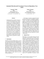
Figure 1: A high-pressure waterjet rapidly bores a hole through the
soil to strike a buried object. The impact of the waterjet with the
buried object creates sounds which are indicative of that object. A
typical antipersonnel mine may be 3


in diameter and buried 2

deep. The microphone and nozzle are typically located 1

–4

above
the soil surface.
types are often weak, making it difficult to differentiate the
plastic landmines from the mineral content of the surround-
ing soil. Due to high sensitivity, an MD very often provides
a false positive signal for small metal debris. GPR sensors
have proven more successful in detecting plastic-cased mines.
However, GPR sensor systems often suffer from high false-
alarm rates since they respond to dielectric discontinuities
in metallic and nonmetallic objects. As a result, there is a
need for confirmation sensors to help resolve false alarms.
Furthermore, the MD- and GPR-based systems provide only
an approximate location for the potential landmines. A con-
firmation sensor such as a metal rod is currently used to pre-
cisely locate the mine. In this paper, waterjet technology is
investigated as a confirmation sensor for landmine location
and discrimination.
A high-pressure waterjet, fired at soil, will quickly create
a borehole in the soil (Figure 1). If the waterjet hits an ob-
ject, the object vibrates, producing a sound that may be used
todetectandevenidentifythatobject[9, 10]. This sound is
a function of the waterjet, its angle with respect to the ob-
ject, the position at which the object is struck, the character-

istics of the surrounding environment (soil cover), and the
physical characteristics of the object like its shape, elasticity,
and mass. The majorit y of energy in the sound is typically in
the range of 2–10 kHz. The total force applied to the object
is small, less than 5 pounds for a waterjet fired at 2500 psi
through a 0.05

nozzle. This force is typically much less than
what is required to set off a landmine. If needed, even less
force can be used by decreasing the pressure or nozzle size.
Depending on pressure, nozzle diameter a nd firing time, the
waterjet can penetrate up to 12

deep [11]. This research in
waterjet-based landmine detection is based on the premise
that the acoustic signal produced by the impingent waterjet
is characteristically different for different types or classes of
objects [9, 10]. Our objective is to show the potential of us-
ing the sound produced by a high-pressure waterjet impact
to detect and classify buried landmines.
Three methods of detecting and classifying a buried ob-
ject using the sound of a waterjet impact were investigated.
The methods were based on (a) using unique features com-
puted f rom the correlation of the recorded sound over time
with weig hted density distribution (WDD) functions, (b) us-
ing a maximum likelihood (ML) estimator applied to the
power spectral density of the recorded signal, and (c) us-
ing a hidden Markov model (HMM) and cepstral coefficients
to model the system as a time-dependent random process
whose spectral characteristics are governed by a first-order

Markov process. A variety of methods to improve the accu-
racy of these techniques were explored. The theory and ra-
tionale behind each of these three methods and their ability
to classify objects are summarized in the following sections.
2. THEORY
2.1. Basis functions applied to temporal acoustic data
The first approach investigated computed temporal features
of the acoustic signal. To quantify the change in acous-
tic signal magnitude over time, correlation of the acoustic
signal magnitude with a set of basis functions was exam-
ined. WDD functions have been applied for computing spa-
tially and temporal ly distributed features in hand-held units
for landmine/no-landmine discrimination from MD signals
[12, 13, 14]. Here, we extend this research to the application
of the WDD functions for determining temporal features
from the magnitude response of an acquired acoustic signal.
The application of the WDD functions to waterjet data is in-
tended to quantify two components of the temporal acous-
tic signal: (1) low frequency content of the acoustic signal
and (2) consistency of the acoustic signal magnitude varia-
tion for different object types over the duration of the acous-
tic response. The temporal features are point-to-point cor-
relations of the WDD functions with the sample-by-sample
magnitude of the acoustic signal.
Figure 2 shows the WDD functions, W
k
(for k =1, ,6),
that were correlated with measured and windowed sound
signals. From Figure 2, the WDD function number is given
in parentheses. Let r[n] represent the windowed sound sig-

nal w ith N total samples (n = 1, , N). The WDD func-
tions are piecewise linear, where the WDD function values
for each piecewise linear segment are adjusted based on the
number of samples (N) to facilitate point-to-point correla-
tion. Let W
k
[n] denote the value of the WDD function at
sample position n. Six WDD features, ( f
1
, , f
6
), are com-
puted as
f
k
=
N

i=1
r[i]W
k
[i](1)
for k = 1, 2, , 6. Six additional features, ( f
7
, , f
12
), are
computed from the absolute difference between consecutive
Landmine Detection and Discrimination Using Waterjets 1975
1

−1
1 N
(1)
1
−1
1 N
(2)
1
−1
1 N
(3)
1
−1
1 N
(4)
1
−1
1 N
(5)
1
−1
1 N
(6)
Figure 2: WDD functions were correlated with acoustic data produced by the waterjet-mine interaction to calculate temporal features of
theacousticdata.
sound values as
f
k
=
N


i=1


r[i] − r[i − 1]


W
k
[i](2)
for k = 7, 8, , 12, where r[0] = 0.
A clustering-based approach was used to discriminate
landmines from soil or harmless objects using the twelve
WDD features. To compute clusters, the sound data collected
at each test site was divided into 10 randomly chosen training
and test sets, using 80% of the data for training and the re-
maining 20% for test (see following sections). K-means clus-
tering [15] of the landmine encounters from the training data
was performed to generate a model representation of land-
mines. The number of clusters, m, was determined empiri-
cally.
The nearest neighbor approach was used for landmine
discrimination [15]. Let D
i
denote the Euclidean distance
from cluster i (1 ≤ i ≤ m), where m is the number of
clusters. Then, D
min
= min(D
1

, , D
m
) represents the min-
imum distance from the feature vector for the current wa-
terjet encounter. D
min
is determined for all landmines and
harmless objects from the training data. Let A ={A
1
, , A
r
}
represent the set of minimum distances for the landmine-
waterjet encounters from the training data to the nearest
landmine cluster, where r is the number of landmine clusters.
Let B ={B
1
, , B
s
} denote the corresponding set of min-
imum distances for the nonlandmine waterjet training en-
counters. The confidence value assigned for each encounter
was assigned as
C
=










1forD
min
<B
min
A
max
−0.5B
min
−0.5D
min
A
max
−B
min
for B
min
≤D
min
<2A
max
−B
min
,
0forD
min
≥ 2A

max
− B
min
,
(3)
where A
max
= max{A
1
, , A
r
} and B
min
= min{B
1
, , B
s
}.
C is assigned the value 1 for distances less than the minimum
distance found for non-landmines (i.e., the encounter was
with a harmless object) and declines linearly to 0 based on
the maximum distance determined for landmines.
2.2. Maximum likelihood applied
to power spectral density
The second approach investigated used the power spectral
density of the sound produced by the waterjet encounter to
detect landmines. This approach is a classic method used to
detect and classify a signal in a noisy, indeterminate environ-
ment. It was tested because it is simple to apply and works
well for a broad set of problems. Probability density func-

tions were generated for the signal power as a function of
frequency for different types of encounters. Object detection
and classification was based on an ML decision.
Previous research has shown that the sampled micro-
phone data, r[n], becomes quasistationary approximately
250 ms after the waterjet is turned on over dry sand [10].
Within the quasi-stationary period, r[n] can be modeled
well as a Gaussian stationary random process [16]. As such,
r[n] can be characterized by its power spectrum, S
r
( f ). The
power spectrum derived from any particular signal will de-
pend on a set of physical parameters, θ,suchasobjecttype,
depth, and soil condition. In discrete form, the probability
density function for a particular parameter set θ
i
is given by
f

x, θ
i

=
1


C
i



1/2
(2π)
k/2
e
−1/2(x−x
i
)
T
C
−1
i
(x−x
i
)
,(4)
where
x =







S
r

f
0


S
r

f
1

.
.
.
S
r

f
k








(5)
1976 EURASIP Journal on Applied Signal Processing
is a vector of measured power spectral density values at dis-
crete frequencies f
0
through f
k
, k is the number of discrete

frequencies available, and x
i
and C
i
are the vector mean and
cross correlation matrix, respectively, of the power spectral
density associated with physical parameter set θ
i
.Forour
tests, the parameters x
i
and C
i
were estimated from calibra-
tion data [17].
A widely accepted solution for the best choice among the
set of simple hypotheses
{H
j
} is given by the hypothesis, H
i
,
for which [17]
f

x, θ
i

≥
f


x, θ
j

∀
j,(6)
where the search space {θ
j
} is defined over all possible phys-
ical parameters that may be encountered in a particular test.
The hypothesis H
i
is an “ML” solution.
Datasets used in this study were small, so principal com-
ponent analysis was used to improve results. In this case [18],
f

x, θ
i

=
1


Λ

i


1/2

(2π)
j/2
e
−1/2(x−x
i
)
T
U

Λ
−1
U
T
(x−x
i
)
,(7)
where U isamatrixofeigenvectors,Λ is a diagonal matrix
of eigenvalues, λ
i
,and
ˆ
C
i
= UΛU
T
. The principal compo-
nents of
ˆ
C

i
are given by the eigenvalues λ
0
, , λ
j
for which
λ
j
>ε,whereε is a constant chosen heuristically. The number
of principal components may vary between parameter sets
for a given constant ε. A change in the number of principal
components causes a fundamental change in the value of the
probability density function. Since the components are or-
thogonal, this change can be seen by the decomposition of
f (x, θ
i
) as the joint probability of individual components λ
j
:
f

x, θ
i

=

j
f
λ
j


x, θ
i

,(8)
where
f
λ
j

x, θ
i

=
1
λ
1/2
j
(2π)
1/2
e
−1/2(x−x
i
)
T
u
j
λ
−1
j

u
T
j
(x−x
i
)
. (9)
Representation of one hypothesis with more principal com-
ponents, j, than another places a more restrictive condition
on the hypothesis with more principal components since the
data must align well along more component directions. To
accurately compare values of probability density between pa-
rameter sets with a different number of principal compo-
nents, the jth root of the probability density function was
taken before comparison. In this way, we are effectively cal-
culating the geometr ic mean among values of the probabil-
ity density function for each principal component and using
that geometric mean to compare hypotheses.
2.3. Hidden Markov model approach
The third approach investigated was based on an HMM of
the dynamics of the waterjet-soil-object interaction. The ob-
servation feature vector for discrimination is based on linear
prediction coefficients and cepstral analysis which captures
the local time-variant spectral characteristics of the waterjet-
soil-object interaction.
The use of HMMs for object detection is motivated
by the characteristics of the waterjet-soil-object interaction.
Figure 1 shows a simple illustration of the waterjet setup and
expected waterjet-soil-object interaction. We describe any
acoustic signal as a combination of three states correspond-

ing to the following ones:
State 1: interaction of jet with soil.
State 2: interaction of the jet with the object (when present).
State 3: decay of the jet.
The presence of the object is dictated by the presence or ab-
sence of State 2. Also, the probability of the presence of the
subsequent state is dependent on the cur rent state of the
model, which is a first-order Markov model. Neither of these
states are visible to the user; the user only hears the acoustic
signal produced. These states show themselves as a function
of the acoustic signal that is picked up by the microphone,
thus the name hidden states, and hidden Markov models.
The HMM for a given object is described in terms of the
probabilities of a state transition from one state to the other
and the probability of the state given an obser vation signal
[19, 20]. These probabilities and hence the HMM’s can be
learned using signals emitted from known objects within cal-
ibration lanes. The first step in defining the HMM is the fea-
ture selection and generation of the observation sequence.
The observation signal is the sound produced by the
waterjet-soil-object interaction during the firing of the wa-
terjet pulse. This raw acoustic signal is reduced to an obser-
vation sequence consisting of multidimensional feature vec-
tors that capture the evolution of the waterjet-soil-object in-
teraction. For the current research we have adopted cepstral
analysis to define the feature vector for the waterjet signal
that is then used by the HMM to classify that signal, though
it is possible that several other feature-extraction tools may
work just as well. Similar features are often used in speech
processing for speech recognition and analysis [19].

Cepstral c oefficients characterize the logarithm of the
amplitude spectrum of the observed signal and are thus bet-
ter suited for our detection problem when compared to the
linear predictive coefficients themselves. The waterjet could
be thought of as a source signal (impact). The recorded
sound at the microphone can be thought of as the response of
the buried object to this waterjet (impact) signal. The char-
acteristic signature of this objec t could then be modeled in
terms of its impulse response b(t). Assuming that the source
signal of the waterjet is s(t), the recorded signal x(t)isgiven
by
x( t)
= b(t)
∗
s(t)+η(t)orX( f ) = B( f )S( f )+N( f ), (10)
where η(t) is an additive noise component which may be due
to the background noise (such as that from the high-pressure
pump) or the waterjet exiting the nozzle. For the purposes of
the current discussion, we will assume that this component
can either be neglected or has been filtered beforehand. Note
that the spectral characteristics of the source signal s(t)are
not fixed and may vary due to factors such as change in wa-
terjet pressure and variation in the standoff distance from the
Landmine Detection and Discrimination Using Waterjets 1977
17131925
28142026
39152127
4 10162228
5 11172329
6 12182430

Figure 3: Plot showing the evolution of feature vectors with time
for the signal produced by the background.
nozzle to the surface and/or object. The quantity of interest
here is the signature of the object modeled by b(t) while the
source signal s(t) could be considered as undesirable noise
which could obscure this signature. The logarithm of the am-
plitude spectrum of the observed signal is given by
log


X( f )


≈ log


B( f )


+log


S( f )


. (11)
Thus, while variation in the spectrum of the source signal
will affect the spectrum of the observed signal in a multi-
plicative manner, the corresponding effec t on the logarithm
of the spectrum is additive. As a result, the cepstral coeffi-

cients are more robust to variations in the source signal.
Figures 3 and 4 show the plot of a sequence of fea-
ture vectors for waterjet-induced signals corresponding to
background-only noise and impact with the mine, respec-
tively. Each subplot in these figures shows the feature vector
r
k
={C
k
, ∆C
k
} over time for each block of the signal that is
processed, where “k”istheblocknumberrangingfrom1to
T (T = 30), where T is the number of overlapping blocks per
squirt, and C
k
and ∆C
k
are the cepstral and delta cepstral co-
efficients for the kth block, respectively. The set of all feature
vectors for a given pulse define the raw observation sequence
R
n
={r
1
, r
2
, , r
T
}, where subscript n represents the nth

squirt. In Figures 3 and 4, feature vectors for each block are
displayed in bottom-to-top, left-to-right order. Each block is
numbered for convenience.
Comparing Figures 3 and 4, we can clearly see the differ-
ences between the shape of the cepstral feature vectors asso-
ciated with the background and the mine. Also note that the
feature vectors are very similar for approximately the first 4
frames which show that the starting por tion of the pulse for
separate firings over different objects share similar character-
istics. This duration may however depend on the depth of the
buried object, waterjet pressure, and other factors.
17131925
28142026
39152127
4 10162228
5 11172329
6 12182430
Figure 4: Plot showing the evolution of feature vectors with time
for the signal produced by a mine (low metal antipersonnel mine).
An HMM is characterized by three sets of probability ma-
trices: the transition probability matrix (A), the observation
probability matrix (B), and a prior probability matrix (Π).
For the current analysis we have assumed that the system al-
ways starts in state “one” so that the prior probability matrix
is fixed. Given the current state, the transition probability
matrix gives the probability of occurrence of the new state.
Also for a given state, the observation probability matrix as-
signs a probability to the occurrence of the new observation
feature vector. In order to avoid computational complexity
associated with continuous observation probability density

functions, the feature vectors in the observation sequence
are often quantized into a set of finite symbols using vector
quantization. The sy mbols are assigned according to a min-
imum distance to the prototype vectors stored in a codebook
(ℵ)[20]. The codebook can be estimated using the avail-
able calibration data. Given the raw observation sequence
R
n
={r
1
, r
2
, , r
T
}, the discrete observation sequence is ob-
tained using vector quantization as O
n
={o
1
, o
2
, , o
T
} so
that
o
k
= VQ

r

k
, ℵ

, o
k
∈ V =

v
1
, v
2
, , v
M

, (12)
where V is the set of all possible observation symbols and op-
erator VQ{r
k
, ℵ} represents the vector quantization process
for the given observation r
k
and the codebook (ℵ).
An HMM for the system with N states and M obser-
vation symbols is parameterized in terms of three prob-
ability matrices A, B,andΠ. We use the notation, Λ =
{A
N×N
, B
N×M
, Π

1×N
} to indicate the complete parameter set
of the model. Given a set of observation sequences for the
system, the HMM parameter Λ ={A
N×N
, B
N×M
, Π
1×N
} can
be estimated using the Baum-Walsh method [19]. In general,
we would expect different Markov models for different types
of buried objects (due to different characteristics of notional
State 2 described earlier).
1978 EURASIP Journal on Applied Signal Processing
Given the HMM for class l, Λ
l
={A
N×N
, B
N×M
, Π
1×N
},
the probability that the observation sequence O
n
=
{o
1
, o

2
, , o
T
} is a result of a first-order Markov process de-
fined by Λ
l
is given by the conditional probability of class l
given Λ
l
and O
n
:
P

l


O
n
, Λ
l

= P

O
n


ˆ
Q

n
, Λ
l

P

ˆ
Q
n


Λ

= π
q
1
T

k=1
b
q
k
o
k
a
q
k−1
q
k
,

(13)
where π
q
1
is the prior probability of state q
1
, b
q
k
o
k
is the prob-
ability of observation o
k
in state q
k
and a
q
k−1
q
k
is the proba-
bility of transition from state q
k−1
to q
k
.
ˆ
Q
n

is the optimal
sequence of states Q
n
={q
1
, q
2
, , q
T
} that maximizes the
conditional probability P(l|O
n
, Λ
l
). Thus,
ˆ
Q
n
= arg max
Q
n

P

l


O
n
, Λ

l

, Q
n
=

q
1
, q
1
, , q
T

. (14)
For waterjet-based detection purposes, an HMM is estimated
for each class of object to be detected. Once the HMM has
been learned for a given class or identity of object (for exam-
ple, a given mine or a given class of mines), a new observa-
tion is said to belong to class l if the conditional probability
p(1|O
n
, Λ
l
) is above some threshold. For a multiclassification
problem, the above conditional probability can be obtained
for each class of objects and the class with highest conditional
probability defines the identity of the buried object. Thus
L = arg max
l


P

l


O
n
, Λ
l

, l ∈{classification}. (15)
3. LABORATORY DATA
Mine detection algorithms were tested both using laboratory
data and field data. Laborator y data was used to test the al-
gorithms’ ability to detect when an object was struck by the
waterjet as opposed to when the waterjet struck only soil or
sand. It is important to be able to distinguish a miss from a
hit so the user knows when an object has been struck and be-
cause a human operator can construct a mental picture of the
object’s size and shape simply by striking the object several
times at different locations (as is often done with a titanium
probe). Such a method could also be very useful for show-
ing if an MD has indicated a large object that is potentially a
mineorasmallbitofmetallicdebris.Fielddatawasusedto
test the algorithms’ ability to classify the type of object struck.
The following section details the methods and results re-
lated to the laboratory data. Field data are discussed after-
wards in another section.
3.1. Methods
Laboratory data was taken from objects buried in a sand-

filled tub, as illustrated in Figure 5. Objects (either a rock
or dummy antipersonnel landmine) were buried approxi-
mately 1.5

below the sand. Objects were approximately 3

to 4

in diameter. The waterjet was fired into the sand ap-
proximately every 2

. Location and firing of the jet was
Figure 5: Data was taken in the laboratory using the setup shown.
Sounds produced by the waterjet-soil-object interaction were
recorded by the microphone on the left. The position and firing of
the waterjet nozzle (right) were controlled by a computer.
controlled automatically through a computer control system.
Sounds were sampled and recorded with 16 bits of preci-
sion at 44.1 kHz using a Peavey cardioid unidirectional mi-
crophone. Water pressure was approximately 3000 psi. The
waterjet w as turned on for approximately 1 second for each
squirt. Nozzle diameter was 0.043

. A total of 29 recordings
were made of a waterjet encounter with an object and 163
of an encounter with only sand. Each recording contained a
single firing of the waterjet.
For testing purposes, 10 sets of test and training data were
prepared from the laboratory data. For each set, 20% of the
data (20% of the object encounters and 20% of sand-only en-

counters) were randomly a llocated for testing and 80% were
allocated for training. The ability of each algorithm to detect
buried objects was measured using these datasets. Results are
reported for the average performance among these sets.
3.2. Results
Receiver operating characteristic (ROC) curves were calcu-
lated for each detection algorithm based on its ability to de-
tect when the waterjet hit an object. ROC curves are given
for the WDD, ML, and HMM approaches in Figure 6.The
probability of false alarm necessary to reach a 90% proba-
bility of detection was 0.18 for the WDD approach, 0.25 for
the maximum likelihood approach, and 0.56 for the HMM
approach.
4. FIELD DATA
Field data was used to determine the ability of the algorithms
to classify the type of object struck by the waterjet. Data was
first taken in calibration lanes, where the t ype of object was
known at each position. This calibration data was used to im-
prove and train our algorithms. Data was next taken in blind
test lanes, where only the approximate position of buried
Landmine Detection and Discrimination Using Waterjets 1979
ML approach
WDD approach
HMM approach
00.20.40.60.81
Probability of false alarm
0.5
0.6
0.7
0.8

0.9
1
Probability of detection
Figure 6: Receiver operating characteristic curve showing the abil-
ity of each approach (ML, WDD, HMM) to detect when the water-
jet struck a buried object. Results are shown for data taken in the
laboratory.
objects was known. Data from the blind test lanes was used
to show the efficacy of the methods. The methods and results
are discussed below. Because each algorithm has its own pe-
culiar strength and weaknesses, the tests and preprocessing
methods applied to the calibration data will differ from one
algorithm to another.
4.1. Hardware
A hand-held “lance,” shown in Figure 7,wasconstructedto
gather field data.
1
The lance was constructed to allow an indi-
vidual deminer to survey the field, giving him great freedom
in the placement and number of test shots used. The lance is
connected through hoses to a high-pressure pump and reser-
voir. A test shot is made every time the deminer presses the
trigger. The length of the shot is controlled by an electronic
timer and a solenoid valve mounted on the lance. Our tests
used a waterjet pressure of 2000–2500 psi, a 0.05

diameter
nozzle, and squirt duration of approximately 1 second. For
this setup, each squirt used approximately 2.2cm
3

of water
and penetrated the soil approximately 6

. The nozzle size
and duration can be reduced to limit water usage, but even
at this volume a deminer could work all day using only a few
gallons of water. Sounds from each squirt were recorded by
a Schoeps CCM41 supercardioid microphone mounted on
the lance arm. Sounds were sampled at 96 kHz using a 24
bit digital-to-analog converter. Before each shot, the wand
was placed firmly on the ground and supported by the tripod
mounts. The angle between the nozzle and ground varied be-
1
The lance was designed by Dr. Grzegorz Galecki and Dr. David Sum-
mers of the UMR Rock Mechanics Laboratory.
tween 30 and 45 degrees. While this firing angle differed from
the angle used in our labor a tory tests shown earlier, prelimi-
nary studies in the laboratory indicate that the angle should
not prevent detection and discrimination. The more shallow
firing angle was required for other tests we performed using
radar as part of another study.
4.2. Calibration and test lanes
Test and calibration lanes were provided for sand and for clay
at a government test facility. Each lane contained 10 buried
objects. Five objects were buried at a particular depth for cal-
ibration and five for test. Objects included 7 types of land-
mines and 3 types of harmless objects, as given in Ta ble 1 .
Landmines were primarily antipersonnel-type mines, usually
with very low metal content, though one antitank mine was
included in the study.

2
Mines ranged in size from antiper-
sonnel mines approximately 3

in diameter to an anti-tank
mine approximately 12

in diameter. No specific object or
mine type was repeated in a particular calibration lane. The
location of each object in the lane was identified with a flag.
The identity of objects next to each flag was given to UMR
for the calibration sites. Test sites were constructed under
the same conditions and from the same objects as calibration
sites, but the object at a particular site was unknown to UMR;
hence there were five “unknown” objects buried at 2

and 4

in both sand and clay (20 unknown objects total). Ob jects
at “blind” test sites were identified for UMR after analysis
was complete. The depths of test objec ts were known for clay
but were unknown for sand (either 2

or 4

as at calibration
sites).
4.3. Data
A total of 52 acoustic signals were collected from calibration
sites for objects as well as five sig nals for the waterjet hitting

only clay (no object clutter) and three signals for sand only
(no object clutter). There were 2 6 waterjet-object encounters
in clay and in sand each. Multiple shots were taken at each
object. After squirting an object in the calibration lane, it was
manually confirmed that the shot actually hit the desired ob-
ject. No confirmation of a hit or miss was taken at blind test
sites, as such confirmation could not be done during actual
demining. At test sites, hits or misses were determined from
the recorded sound using our a lgorithms. For this reason, it
is possible that some recordings at test sites were classified as
hitting an object when, in fac t, they did not. This possibil-
ity may skew classification results shown later, but is true to
what would occur during an ac tual demining operation.
4.4. Preprocessing and filtering of the acoustic signal
When the waterjet is fired, a low frequency vibration is in-
duced in the wand due to the opening and closing of the wa-
terjet v alve. This vibration is picked up by the microphone
due to its high sensitivity. This low-frequency vibration was
2
An agreement with our sponsor prevents us from specifying the precise
mines used in the study.
1980 EURASIP Journal on Applied Signal Processing
Tri gger
Hose to
pump
Solenoid
valve
Nozzle
Microphone
Figure 7: The waterjet lance used to collect data in the field.

Table 1: Type of object located at each flag position in field calibration lanes.
Flag number 2

sand calibration lane 4

sand calibration lane 2

clay calibration lane 4

clay calibration lane
1 Antipersonnel Antipersonnel Metal disc Metal disc
2 Antipersonnel Plastic disc Plastic disc Plastic disc
3 Wood block Antipersonnel Antipersonnel Wood block
4 Antipersonnel Metal disc Antipersonnel Antipersonnel
5 Antipersonnel Antipersonnel Antitank Antipersonnel
found to be additive with sounds picked up by the micro-
phone so that we were able to filter away this contribution.
A high pass 2048-tap FIR filter with a cutoff frequency of
100 Hz was used to remove this signal. Since our tests indi-
cate there is typically no useful information in the frequency
range of approximately 0–120 Hz, we were able to do this pre-
processing without any loss of useful information.
4.5. Object classification
Data from calibration sites was used to train each classifica-
tion approach and determine optimal processing methods.
Once training was complete, the approaches were used to
classify the sounds from the blind test sites. Identity of the
objects at blind test sites was revealed to the authors after
classification was complete. A discussion of the results of
training and optimizing algorithms using calibration data

follows.
4.5.1. WDD approach—calibration
Two classification approaches were investigated. First, indi-
vidual models were developed for sand and for clay based on
a K-means, nearest-neighbor-based discriminator. Second,
a single model were developed that combined the clay and
sand encounters into a single dataset. Experiments were per-
formed to compare classification results using the two mod-
els. For the separate models, the 2

and 4

sand calibration
data was used to train a WDD “sand + landmine” model.
Likewise, the 2

and 4

clay calibration landmine encounters
was used to train a WDD “clay + landmine” model. Soil-only
encounters were used to normalize data within each soil type.
Data was normalized by subtracting the mean of the soil-only
encounter for the specific soil type and dividing by the stan-
dard deviation. WDD features were computed from the nor-
malized data. For the combined-soil-type model, the sand
and clay encounters were combined to generate one dataset
from which the WDD landmine model was developed. For
the combined-soil type, the means and standard deviations
determined from the sand-only and clay-only data were used
to normalize the respective sand and clay data. For evaluation

purposes, all landmine encounters were used for training.
During testing, the Euclidean distance to the nearest repre-
sentative landmine cluster was calculated for each encounter.
Distances were used to classify objects as harmless or as land-
mines. ROC curves were used to evaluate results.
Experimental results showed that the combined-soil
model discriminated between landmines and harmless ob-
jects better than the separate-soil models did. However, the
overall landmine classification rates were poor. Setting the
threshold to achieve 100% correct landmine recognition
yielded 27.7% correct harmless object classification. Setting
the threshold to achieve 62.0% correct landmine classifica-
tion yielded 83.3% correct harmless object classification.
Experimental results for the combined soil model showed
that classification rates for the first squirt at each object
were much better than for the remaining squirts. Specif-
ically, classification using the first encounter at each flag
position yielded 92.3% correct landmine recognition with
72.7% correct harmless object recognition. The first shot
may be a better predictor because each shot causes some
changes to the soil conditions that are reflected in the sounds
Landmine Detection and Discrimination Using Waterjets 1981
Table 2: Percentage objects correctly identified in field calibration dataset using ML approach. In this case, the test data was taken from the
same dataset used to form test statistics.
Percent correctly identified
Preprocessing method
Grouping 1 Grouping 2 Grouping 3
soil, object, depth object typ e mine/harmless
None 19% 37% 53%
Normalize 11% 47% 83%

Log 10% 25% 92%
Normalize and Log 12% 24% 93%
produced on subsequent firings. Accordingly, the following
approach was used for classifying the blind test encounters.
The combined-soil WDD feature-based landmine model was
used. Test data was normalized as before. The first encounter
or squirt at each flag location was used as the basis for the
landmine/harmless object classification decision. The same
distance thresholds were used to classify test data as with cal-
ibration data. If the Euclidean distance was less than or equal
to the threshold, the encounter would be labeled as a land-
mine. Otherwise, the encounter was called a harmless object.
If the encounter was labeled as a landmine, the type of land-
mine assigned to the encounter would simply be the land-
mine type from the calibration encounters with the closest
Euclidean distance. If the encounter was labeled as a harm-
less object, the type of harmless object assigned to the en-
counter would simply be the harmless object type from the
calibration encounters with the closest Euclidean distance.
4.5.2. Maximum likelihood approach—calibration
The maximum likelihood approach allows a grouping of data
types that may be difficult to obtain with the other classifica-
tion techniques. Since our calibration data was limited, the
ability to form larger groups that may be independent of one
or more physical parameters (for example depth or soil type)
may allow the for mation of better test statistics. Several pos-
sible groupings of the data were tested.
(i) Grouping 1. Data was grouped according to soil type
(sand, clay), specific identity, and depth. For example,
encounters with a wooden block buried at 2


in sand
would be used to generate one set of statistics. Encoun-
ters with a wooden block buried at 4

in sand would be
used to generate another. Results thus included identi-
fication of the object, depth, and soil type. In this case,
objects were classified as belonging to one of 20 differ-
ent groups.
(ii) Grouping 2. Data was grouped together according to
object type (e.g., wood block versus plastic plate), re-
gardless of the depth of the object or the type of soil
the object was placed in. Objects were classified as be-
longing to one of 11 different groups.
(iii) Grouping 3. Data was grouped into two classes, land-
mine or harmless object.
Optimal preprocessing of data may also improve results.
Three methods of preprocessing the data before application
of the ML approach were tested: ( a) normalization of the
power spectral density such that the integral of power spec-
tral density evaluated to one for each measured signal, (b)
taking the log of the power spectral density, and (c) first nor-
malizing and then taking the log of the power spectral den-
sity. These techniques were also compared to the case where
no preprocessing was done.
All available calibration data was used for initial train-
ing and testing. Calibration tests should still reflect perfor-
mance reasonably well since data is represented statistically
using only a few components and thus the approach cannot

“memorize” the training set. Test signals were associated with
a group according to whichever group had the highest-valued
probability density function as shown in (4).
Results for the calibr ation dataset are shown in Table 2.
The ML approach was able to correctly classify 93% of ob-
jects as harmless or harmful by normalizing and taking the
log of data and was able to predict the object identity with up
to a 47% accuracy by normalizing data before processing.
4.5.3. HMM approach—calibration
To make the estimation of LPC/cepstral coefficients less noisy
and more representative of the desired signal, the original
44.1 kHz raw data were downsampled to a 6000 Hz signal.
Earlier analysis has shown that the discriminatory informa-
tion is predominantly in the lower frequency spectrum of the
waterjet-induced acoustic signal. Up to 8th-order LPC coef-
ficients were used for the feature vector so that the resulting
feature vector was 22-dimensional.
As discussed earlier, a discrete HMM with finite observa-
tion symbols describing three states was used. A major issue
in vector quantization was the design of an appropriate code-
book for quantization. After some trials we found a code-
book size of 64 to be appropriate for this application (i.e.,
there were 64 possible observations in each state). A larger
codebook was not possible because we were working with a
very limited dataset. Separate codebooks were designed for
different soil conditions and different depths. To design the
codebook, we selected an equal number of raw observation
sequences corresponding to mines and harmless objects. The
feature vectors for all these observations were concatenated
and passed on as a representative training sequence to a pro-

gram that designs the codebook using a K-means segmenta-
tion algorithm [21]. A Euclidean distance metric was used in
the generation of the codebook and for code assignment.
1982 EURASIP Journal on Applied Signal Processing
Table 3:Percentageofobjectscorrectlyclassifiedasharmfulorharmlessatblindfieldtestsites.
WDD prediction ML prediction HMM prediction Observer
Sand, mixed depth 50% 50% 40% 90%
Soil, 2

depth 60% 60% 60% 60%
Soil, 4

depth 60% 60% 20% 60%
Table 4: Percentage of objects correctly identified (e.g., a wooden block or a rock) at blind field test sites.
WDD prediction ML prediction HMM prediction Observer
Sand, mixed depth 20% 10% 10% 70%
Soil, 2

depth 20% 20% 40% 40%
Soil, 4

depth 20% 20% 20% 20%
A separate HMM was trained for each desired classifica-
tion of the targets. The calibration dataset was used to train
these HMMs. The following are the steps involved in the
training of the discrete HMMs.
(1) The number of states in our model was kept fixed at
N
= 3.
(2) The transition matrix and the observation matrix were

randomly initialized. The a priori probabilities of the
states were initialized to Π ={1, 0, 0}, forcing the con-
dition that the HMM always started in State 1.
(3) All squirts corresponding to the given class were se-
lected and the corresponding observation sequence
was obtained.
(4) The quantized observation sequence was used to t rain
the state transition matrix and observation matr ix
starting from the randomly initialized parameters u s-
ing the Baum-Walsh method [19].
(5) Since the HMM parameter estimation may be trapped
in local minima, we performed the training routine
many times (with different initial conditions) and
chose the model that had the maximum mean likeli-
hood ratio.
Mine detection and classification was carried out at two lev-
els. First, each squirt from the waterjet was classified as hit-
ting either a mine or harmless object. Three separate HMMs
were trained using calibration data for each class and each
dataset. Second, after classifying the data into the classes of
mine and harmless object, we proceeded to try and iden-
tify the target type (from among the seven mine types and
three harmless object types) present in each data class. In
this case the signals from each dataset were classified based
on their target identity and separate HMMs were trained for
each target type. For the soil calibration data at 2

this re-
sults in 5 classes (4 mine types, one harmless object). Sim-
ilarly for the soil calibration data at 4


we created 5 classes
and the sand calibration data generated 8 classes. After train-
ing, the HMMs were tested on the dataset on which they were
trained, to check if they had been trained properly.
When testing the HMMs using the calibr ation training
set, the HMM approach was able to correctly identify 100%
of sounds as associated with a mine or harmless object and
was able to correctly predict the target identity for 92% of
the sounds. These results indicate that the training was ac-
complished effectively.
4.5.4. Blind test site results
Sounds at the blind test sites were classified using the WDD,
ML, and HMM approaches as given in the previous sections.
Tabl e 3 shows the percentage of objects correctly classified
as harmful or harmless for each technique. The percentage
of objects whose specific identity (e.g., wooden block as op-
posed to rock) was correctly predicted by the algorithms is
given in Ta ble 4. These tables also include the performance
of a human observer who participated in the tests and made
predictions about the mine type based on what they heard or
saw. The human observer did not know which object was be-
ing st ruck until after results had been compiled and the tests
were complete.
5. DISCUSSION AND CONCLUSIONS
The goal of this study was to show the potential of using the
sound produced by the impact of a high-pressure w aterjet
to detect and classify bur ied landmines. Previous work had
shown this possibility existed, but did not show a clear route
toward achieving accurate classification [9, 10]. In the ab-

sence of additional direction, three methods based on the
temporal (WDD), spectral (ML), and a combination of tem-
poral and spectral (HMM) characteristics were attempted.
Results with laboratory data suggest the low-frequency vari-
ation of the sound signal over time is a better indication
of when the waterjet hit or missed a buried object, as the
WDD approach slightly outperformed the other approaches
in this case. All three approaches performed similarly when
attempting to classify buried objects in field experiments.
The comparison in the field is a bit weak, however, due to the
small quantity of data available. A clear picture of the charac-
teristics in the sound that best identifies the buried object is
still in question. The presence of these characteristics is indi-
cated by the performance of the human observer in our tests.
Finding these characteristics remains for future studies.
Landmine Detection and Discrimination Using Waterjets 1983
Classification techniques performed well when identify-
ing whether the waterjet struck an object or hit only soil (i.e.,
identifying a hit/miss or object/no-object). Techniques also
performed well with calibration training data when classify-
ing encounters as with a mine or harmless object or identify-
ing the object, but performed poorly when using data from
the blind test sites. Poor performance at the blind test sites
was probably related to the quantity and quality of calibra-
tion data. Each technique requires a fair amount of calibra-
tion data for appropriate training. The amount of training
and test data available from our field study was relatively
small. With more data, we would expect better performance.
It is interesting to note that the human observer was gen-
erally able to classify waterjet signals better than our signal

processing algorithms, at least when classifying the object
struck by the waterjet. Humans have an amazing ability to
recognize patterns in audio signals. They also have the ad-
vantage that they may incorporate visual information into
their decision, such as the location of each hit or miss when
interrogating a buried object. The performance of the human
observer indicates that there is additional information in the
waterjet data that has not been exploited by our algorithms.
Recognizing this information is a key to improving results.
The preprocessing methods and classification techniques
used in these experiments were formed heur istically. Better
results could be expected if techniques were based on the
physics behind sound production. Sounds from the water-
jet/object impact are a function of the interaction of the wa-
terjet and object, the physical characteristics of the object, the
surrounding media, the borehole created by the waterjet, and
more. Understanding how sounds recorded by the micro-
phone were produced would improve our ability to process
data and extract identifying information. This understanding
could be used to develop “filters” to remove unwanted infor-
mation and produce measures related to the physical charac-
teristics of the object.
In our tests, objects were classified by separately classi-
fying the sounds from each individual squirt. The ML ap-
proach could easily be extended to make decisions based on
all the squirts at an object, rather than each squirt separately.
If the sounds made by a squirt at an object is independent of
other squirts, then the joint probability density function for
these sounds is given by
f


x
1
, x
2
, , x
k
, θ
i

= f

x
1
, θ
i

f

x
2
, θ
i

··· f

x
k
, θ
i


, (16)
where f ( x
1
, θ
i
) is the probability density function for an in-
dividual squirt on object i. For the set of sounds {x
k
}, the ML
prediction is given by the hypothesis, H
i
,forwhich
f

x
1
, x
2
, , x
k
, θ
i

≥ f

x
1
, x
2

, , x
k
, θ
j

∀ j. (17)
Using all the shots over a single object to identify the object
within the calibration set improved identification of the ob-
ject from 47% (single-shot classification) to 57%.
Using a waterjet to detect and classify bur ied objects is a
unique approach to demining. Hits or misses were classified
in laboratory data with more than a 90% probability of de-
tection while achieving less than a 20% false-alarm rate. The
type of object was correctly classified in up to 100% of cases
when using calibration data and up to 60% of cases using
blind test data. Results in the field were best with a human
observer, who was able to classify objects with up to 90% ac-
curacy. While better detection is needed for actual demining
purposes, these preliminary results show the promise of the
waterjet approach. Future research into the mechanisms that
generate the sounds and into refinement of our classification
algorithms should yield better results. The waterjet may be
particularly useful as a confirmation sensor used with other
sensors, like an MD. In this case, the ability to quickly and
safely discern the size of a buried object or whether the ob-
ject is harmful or harmless could significantly improve the
demining process.
ACKNOWLEDGMENT
The authors gratefully acknowledge the help of Robert De-
nier, Grzegorz Galecki, Tom Herri ck, Robert Mitchell, and

David Summers who helped collect data, design, and manu-
facture test equipment, and who have been long-term partic-
ipants in the overall project.
REFERENCES
[1] C. Bruschini and B. Gros, “A survey on sensor technology for
landmine detection,” Journal of Humanitarian Demining, vol.
2, no. 1, 1998.
[2] J.MacDonald,J.R.Lockwood,J.McFee,etal.,Alternatives for
Landmine Detection, RAND, Santa Monica, Calif, USA, 2003.
[3] L. Carin, Ed., “Special issue on landmine and UXO detection,”
IEEE Transactions on Geoscience and Remote Sensing, vol. 39,
no. 6, 2001.
[4] E. Cespedes and D. Daniels, Eds., “Special issue on UXO and
mine detection,” Subsurface Sensing Technologies and Applica-
tions, vol. 2, no. 3, 2001.
[5] K. Bruschini, C. De Bruyn, H. Sahli, and J. Cornelis, “EU-
DEM: The EU in humanitarian DEMining—Final Report,”
1999, />[6] N. Milisavljevic, “Comparison of three methods for shape
recognition in the case of mine detection,” Pattern Recognition
Letters, vol. 20, no. 11–13, pp. 1079–1083, 1999.
[7] N. Milisavljevic, I. Bloch, and M. Acheroy, “Modeling, com-
bining, and discounting mine detection sensors within the
Dempster-Shafer framework,” in Detection and Remediation
Technologies for Mines and Minelike Targets V, vol. 4038 of
Proceedings of SPIE, pp. 1461–1472, Orlando, Fla, USA, April
2000.
[8] N. Milisavljevic, I. Bloch, and M. Acheroy, “Characteriza-
tion of mine detection sensors in terms of belief functions
and their fusion, first results,” in Proc. IEEE 3rd International
Conference on Information Fusion (FUSION ’00), vol. 2, pp.

THC3/15–THC3/22, Paris, France, July 2000.
[9] R. Denier, “A heuristic approach to landmine detection us-
ing pulsed waterjet excitation,” M.S. thesis, University of
Missouri-Rolla, Rolla, Mo, USA, 1999.
[10] J. A. Stuller, S. J. Qiu, and K. Das, “Signal processing for land
mine detection using a waterjet,” in D etection and Remedia-
tion Technologies for Mines and Minelike Targets IV, vol. 3710
of Proceedings of SPIE, pp. 1330–1342, Orlando, Fla, USA,
1999.
1984 EURASIP Journal on Applied Signal Processing
[11] D. A. Summers, Waterjetting Technology, E & FN Spon, Lon-
don, UK, 1995.
[12] R. J. Stanley, P. D. Gader, and K. C. Ho, “Feature and decision
level sensor fusion of e lectromagnetic induction and ground
penetrating radar sensors for landmine detection with hand-
held units,” Information Fusion, vol. 3, no. 3, pp. 215–223,
2002.
[13] R. J. Stanley, S. Somanchi, and P. D. Gader, “Impact of
weighted density distribution function features on land mine
detection using hand-held units,” in Detection and Remedia-
tion Technologies for Mines and Minelike Targets VII, vol. 4742
of Proceedings of SPIE, pp. 892–902, Orlando, Fla, USA, April
2002.
[14]R.J.Stanley,N.Theera-Umpon,P.D.Gader,S.Somanchi,
and D. K. Ho, “Detecting landmines using weighted density
distribution function features,” in Signal Processing, Sensor
Fusion, and Target Recognition X, vol. 4380 of Proceedings of
SPIE, pp. 135–141, Orlando, Fla, USA, April 2001.
[15] J. M. Zurada, Introduction to Artificial Neural Systems,West
Publishing, Boston, Mass, USA, 1992.

[16] S. J. Qiu, “Acoustic landmine detection,” M.S. thesis, Univer-
sity of Missouri-Rolla, Rolla, Mo, USA, 1999.
[17] V. K. Madisetti and D. B. Williams, Eds., The Digital Signal
Processing Handbook, CRC Press, Boca Raton, Fla, USA, 1997.
[18] L. L. Scharf, StatisticalSignalProcessing:Detection,Estima-
tion, and Time Series Analysis, Addison-Wesley, New York,
NY, USA, 1990.
[19] L. R. Rabiner, “A tutorial on Hidden Markov Models and se-
lected applications in speech recognition,” Proceedings of the
IEEE, vol. 77, no. 2, pp. 257–286, 1989.
[20] L. R. Rabiner and R. W. Shafer, Digital Processing of Speech
Signals, Prentice-Hall, Englewood Cliffs, NJ, USA, 1978.
[21] Y. Linde, A. Buzo, and R. Gray, “An algorithm for vector quan-
tizer design,” IEEE Trans. Communications,vol.28,no.1,pp.
84–95, 1980.
Daryl G. Beetner is an Associate Profes-
sor of electrical and computer engineering
at the University of Missouri, Rolla. He re-
ceived his B.S. degree in electrical engineer-
ing from Southern Illinois University at Ed-
wardsville in 1990. He received an M.S. and
Doctor of Science degree in electrical engi-
neering from Washington University in St.
Louis in 1994 and 1997, respectively. He
conducts research on a wide range of top-
ics including electrocardiology, skin cancer detection, humanitar-
ian demining, and electromagnetic compatibility.
R. Joe Stanley received the B.S.E.E. and
M.S.E.E. degrees in electrical engineering
and a Ph.D. degree in computer engineer-

ing and computer science from the Uni-
versity of Missouri-Columbia. As a gradu-
ate student at the University of Missouri-
Columbia, he worked under training grants
from the National Library of Medicine and
the National Cancer Institute. Upon com-
pleting his doctoral study, he served as Prin-
cipal Investigator for the Image Recognition Program at Systems &
Electronics, Inc. in St. Louis, Mo. He is currently an Assistant Pro-
fessor in the Department of Electrical and Computer Engineering
at the University of Missouri-Rolla. His research interests include
signal and image processing, pattern recognition and automation.
Sanjeev Agarwal completed his Ph.D. in
Electrical and Computer Engineering from
University of Missouri-Rolla in 1998 and
BTech and MTech degrees (1993) from In-
dian Institute of Technology, Bombay. Dr.
Agarwal joined the Department of Electri-
cal and Computer Engineering at University
of Missouri-Rolla in 1998 and is now a Re-
search Assistant Professor there. Dr. Agar-
wal’s research interests include machine vi-
sion, intelligent computing, image processing, multisensor fusion,
automatic detection theory, airborn e terrain analysis and recon-
naissance, and virtual and augmented reality.
Deepak R. Somasundaram received his B.S.
in electronics and communications engi-
neering from University of Madras, India
in May 2001. He joined the University of
Missouri-Rolla in fall 2001 as a graduate

student of electrical engineering, w here he
worked with Dr. Sanjeev Agarwal on auto-
matic target detection using hidden Markov
models. Currently Deepak is a DSP Engi-
neer with Phonic Ear. His current research
includes adaptive acoustic feedback cancellation and DSP hardware
implementations.
Kopal Nema obtained her B.S. degree in electronics and telecom-
munications from Pune University, India and received an M.S. de-
gree in computer engineering from University of Missouri-Rolla in
May, 2003. She has previously worked as a software engineer for
Cisco. She is currently working with Intel in Bangalore, India.
Bhargav Mantha received the B.S. degree in electrical and electron-
ics engineering from Chaitanya Bharati Institute of Technology, Os-
mania University, in June 2001 and his M.S. degree in electrical en-
gineering from University of Missouri-Rolla in August, 2003. He
now works with Credit Suisse First Boston in New York, USA.