EURASIP Journal on Applied Signal Processing 2003:12, 1167–1180
c 2003 Hindawi Publishing Corporation

Spatially Adaptive Intensity Bounds
for Image Restoration
Kaaren L. May
Snell and Wilcox Ltd., Liss Research Centre, Liss Mill, Mill Road, Liss, Hampshire, GU33 7BD, UK
Email:

Tania Stathaki
Communications and Signal Processing Group, Department of Electrical and Electronic Engineering,
Imperial College London, London SW7 2BT, UK
Email:

Aggelos K. Katsaggelos
Department of Electrical and Computer Engineering, Northwestern University, Evanston, IL 60208-3118, USA
Email:
Received 9 December 2002 and in revised form 24 June 2003
Spatially adaptive intensity bounds on the image estimate are shown to be an effective means of regularising the ill-posed image
restoration problem. For blind restoration, the local intensity constraints also help to further define the solution, thereby reducing
the number of multiple solutions and local minima. The bounds are defined in terms of the local statistics of the image estimate
and a control parameter which determines the scale of the bounds. Guidelines for choosing this parameter are developed in the
context of classical (nonblind) image restoration. The intensity bounds are applied by means of the gradient projection method,
and conditions for convergence are derived when the bounds are refined using the current image estimate. Based on this method,
a new alternating constrained minimisation approach is proposed for blind image restoration. On the basis of the experimental
results provided, it is found that local intensity bounds offer a simple, flexible method of constraining both the nonblind and blind
restoration problems.
Keywords and phrases: image resolution, blur identification, blind image restoration, set-theoretic estimation.

1.

INTRODUCTION

In many imaging systems, blurring occurs due to factors such
as relative motion between the object and camera, defocusing of the lens, and atmospheric turbulence. An image may
also contain random noise which originated in the formation
process, the transmission medium, and/or the recording process.
The above degradations are adequately modelled by a linear space-invariant blur and additive white Gaussian noise,
yielding the following model:
g = h ∗ f + v,

(1)

where the vectors g, f, h, and v correspond to the lexicographically ordered degraded and original images, blur, and
additive noise, respectively, which are defined over an array of pixels (m, n). The two-dimensional convolution can
be expressed as h ∗ f = Hf = Fh, where H and F are

block-Toeplitz matrices and can be approximated by blockcirculant matrices for large images [1, Chapter 1].
The goal of image restoration is to recover the original image f from the degraded image g. In classical image
restoration, the blur is known explicitly prior to restoration.
However, in many imaging applications, it is either costly
or physically impossible to completely characterise the blur
based on a priori knowledge of the system [2]. The recovery
of an image when the blur is partially or completely unknown
is referred to as blind image restoration. In practice, some information about the blur is needed to restore the image.
There are a number of factors which contribute to the
difficulty of image restoration. The problem is ill posed in
the sense that if the image formation process is modelled in
a continuous, infinite-dimensional space, then a small perturbation in the output, that is, noise, can result in an unbounded perturbation of the least squares solution of (1) for
the image or the blur [1]. Although the discretised inverse
problem is well posed [3], the ill-posedness of the continuous



1168
problem leads to the ill-conditioning of H or F. Therefore,
direct inversion of either matrix leads to excessive noise amplification, and regularisation is needed to limit the noise in
the solution.
The blind image restoration problem is also ill defined,
since the available information may not yield a unique solution to the corresponding optimisation problem. Even if a
unique solution exists, the cost function is, with the exception of the NAS-RIF algorithm [4], nonconvex, and convergence to local minima often occurs without proper initialisation. Undesirable solutions can be eliminated by incorporating more effective constraints.
In this paper, spatially adaptive intensity bounds are
therefore proposed as a means of (1) regularising the illposed restoration problem; and (2) limiting the solution
space in blind restoration so as to avoid convergence to undesirable solutions. The bounds are implemented in the framework of the gradient projection method proposed in [5, 6].
Prior research on spatially adaptive intensity bounds
has been conducted solely in the context of classical image
restoration. Local intensity bounds were first introduced in
[7] for artifact suppression. These bounds were applied to
the Wiener filtered image, that is, they were applied to a solution rather than to the optimisation problem itself. In [8], it
was shown that the constraints could be incorporated in the
Kaczmarz row action projection (RAP) algorithm [9]. However, optimality in a least squares sense is guaranteed only if
the constraints are linear [8]. Alternatively, a quadratic cost
function subject to a convex constraint Ꮿ is minimised by
projecting each iteration of the steepest descent algorithm
onto the constraint provided that the step size lies within a
specified range [5]. In [10], space-variant intensity bounds
were applied using this gradient projection method. The intensity bounds were updated using information from the
current image estimate, but the effect of bound update on
the convergence of the gradient projection method was not
analysed. Similar methods have been proposed for the update
of the regularisation parameter and/or the weight matrix in
constrained least squares restoration [11, 12]. In these cases,

convergence was proven via the linearisation of the problem.
The work presented in this paper builds on previous research in several respects [13, 14, 15]. In Section 2, a new
method of estimating spatially adaptive intensity bounds is
proposed. This method is distinguished both in terms of
which parameters define the bounds and, as discussed in
Section 4, how the bounds are updated from the current image estimate. In Section 3, the effect of the scaling parameter, which plays a similar role to the regularisation parameter in classical image restoration, is examined. In Section 4,
convergence of the modified gradient projection method is
discussed. The problem definition changes slightly each time
the bounds are updated, and it is therefore important to understand how this may affect the convergence of the algorithm. Lastly, in Section 5, these intensity bounds are applied
to blind image restoration. A new alternating minimisation
algorithm is established for this purpose. Section 6 contains a
discussion of the results, conclusions, and directions for further research.

EURASIP Journal on Applied Signal Processing
2.
2.1.

DEVELOPMENT AND IMPLEMENTATION
OF LOCAL INTENSITY BOUNDS
Characterisation of the image

It is assumed that the estimated image f belongs to the space
l2 (Ω) of square-summable, real-valued, two-dimensional sequences defined over a finite subset Ω ⊂ P 2 , where P 2 P ×P
denotes the Cartesian product of nonnegative integers [7].
The associated Hilbert space is
Ᏼ

f : f ∈ l2 (Ω) ,

(2)


with inner product and norm
f1 , f2

f1 (m, n) f2 (m, n),
(m,n)∈Ω

(3)

f1 = f1 , f1

1/2

,

for f1 , f2 ∈ Ᏼ.
Typical constraints on the image estimate include nonnegativity and, in blind image restoration, finite support.
In this section, spatially adaptive intensity bounds are combined with these constraints to define the solution space for
the restored image more precisely, leading to better estimates
of both the original image and the blur. Because these constraints define convex sets, they can be incorporated via projection methods. Additionally, a regularisation term [16] is
included in the cost function and can be adjusted to give the
image a desired degree of smoothness.
In any image restoration scheme, there is a trade-off between noise suppression and preservation of high-frequency
detail, since noise reduction is achieved by constraining the
image to be smooth. However, because the human visual system is more sensitive to noise in uniform regions of the image
than in areas of high spatial activity [17], space-variant image constraints may be used to emphasise noise reduction in
the flat regions, and preservation of detail in edge and texture
regions [5, 7, 18, 19]. This is achieved by making the radius
of the bounds proportional to the spatial activity, measured
by an estimate σ 2 (m, n) of the variance of the original imf

age. The local variance is more robust to noise than gradientbased edge detectors [19].
The local mean estimate M f (m, n) is used as the centre of
the bounds. Consequently, the intensity bounds average out
zero-mean noise in regions of low variance.
The local statistics are estimated from the degraded image over a square window centred at pixel (m, n):
M f (m, n) = Mg (m, n) =

1
g(r, s),
Λ r =m−N:m+N

(4)

s=n−N:n+N

1
2
2
σg (m, n) =
g(r, s) − M f (m, n) ,
Λ r =m−N:m+N

(5)

σ 2 (m, n)
f

(6)

s=n−N:n+N


2
2
= max 0, σg (m, n) − σv ,

2
where Λ = (2N + 1)(2N + 1) and σv is the estimated noise


Spatially Adaptive Intensity Bounds for Image Restoration
variance. The window size over which the local statistics are
calculated may be fixed or adaptive [20, 21], but the improvement offered by an adaptive window was found to be
marginal, and a fixed window of size 3 × 3 or 5 × 5 produced
good results.
The proposed intensity bounds are then defined by
f (m, n) − M f (m, n) ≤ βσ 2 (m, n),
f

(7)

1169
blurred image [22]. The regularisation term of (12) is sometimes modified for spatially adaptive noise smoothing by using a weighted norm [5]
Cf

2
W

f ∈ Ᏼ : l(m, n) ≤ f (m, n) ≤ u(m, n),
(m, n) ∈ ᏿ f , f (m, n) = 0, (m, n) ∈ ᏿ f ,
/


(8)

where ᏿ f ⊆ Ω is the support of the image, and
l(m, n) = max 0, M f (m, n) − βσ 2 (m, n) ,
f
u(m, n) = M f (m, n) + βσ 2 (m, n).
f

γ f1 (m, n) + (1 − γ) f2 (m, n)
≥ γl(m, n) + (1 − γ)l(m, n) = l(m, n),
γ f1 (m, n) + (1 − γ) f2 (m, n)
≤ γu(m, n) + (1 − γ)u(m, n) = u(m, n).

(10)

The closure of Ꮿ f follows from the openness of the complement Ꮿcf .
The corresponding projection operator is
P f f (m, n)

=

w(m, n) =

1
,
1 + νσ 2 (m, n)
f

(14)


2
and ν = 1000/σmax is a tuning parameter designed so that
w(m, n) → 1 in the uniform regions and w(m, n) → 0 near
the edges.
The unique solution of (12) is obtained by means of the
following iteration [5, 24]:

fk+1 = P f

(9)

The convexity of Ꮿ f is easily proven by observing that for
any f1 , f2 ∈ Ꮿ f and 0 ≤ γ ≤ 1,

(13)

(m,n)∈Ω

where the weights w(m, n) are calculated according to [18,
21, 23, 24]:

where β is the scaling parameter. Combining the bounds with
the support and nonnegativity constraints yields
Ꮿf

2

w(m, n) c(m, n) ∗ f (m, n) ,


I − αµC T C fk + µH T g − H fk

(15)

= P f G fk ,

where the step size µ satisfies
0<µ<

2
λmax

(16)

and λmax is the maximum eigenvalue of (H T H + αC T C).
Equation (15) represents the projection of the steepest descent iterate onto the constraint Ꮿ f , and hence is named the
gradient projection method.
The iterations are terminated when the following condition is satisfied [1, Chapter 6]:
fk+1 − fk
2
fk

2

≤ δ,

(17)

where δ is typically ᏻ(10−6 ).



l(m, n),








f (m, n) < l(m, n), (m, n) ∈ ᏿ f ,


u(m, n),







f (m, n) > u(m, n), (m, n) ∈ ᏿ f ,

f (m, n), l(m, n) ≤ f (m, n) ≤ u(m, n), (m, n) ∈ ᏿ f ,

0,

(m, n) ∈ ᏿ f .
/
(11)


2.2. Constrained minimisation via the gradient
projection method
The restored image is given as the solution of the following
constrained optimisation problem:
Minimise g − H f

2

2

+ α Cf ,

f ∈ Ꮿf ,

(12)

where α and C are the regularisation parameter and highpass regularisation operator, respectively. In the absence of
local intensity constraints, a rough estimate of α is given
by 1/BSNR, where BSNR is the signal-to-noise ratio of the

3.

CHOICE OF THE SCALING PARAMETER

The scaling parameter β in (9) plays a similar role to the
regularisation parameter α in the classical constrained least
squares approach [16]. If β is too large, then the intensity
bounds fail to prevent noise amplification. However, if β is
very small, then much detail is lost.

In this section, an optimal value of the bound scaling parameter is chosen by maximising the improvement in signalto-noise ratio (ISNR) of the restored image in terms of β,
when α is constant. The ISNR is defined as



ISNR = 10 log 



(m,n)∈᏿ f
(m,n)∈᏿ f

2
f (m, n) − g(m, n) 
2 .
f (m, n) − f (m, n) 

(18)

The effects of the noise level, blur type, and image characteristics are used to develop guidelines for choosing β when
the original image f is unavailable for comparison with the
restored image f.


1170

EURASIP Journal on Applied Signal Processing

(a) Original.


(c) Restoration using uniform
regularisation: ISNR = 0.90 dB.

(b) Degraded.

(d) Restoration using additional local
bounds: ISNR = 2.15 dB.

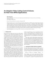
Figure 1: Restoration of Cameraman image, degraded by 1 × 9 Gaussian blur, BSNR = 20 dB.

To illustrate the effect of β on the ISNR, the 256 × 256
Cameraman image in Figure 1a was degraded by a 1 × 9 point
spread function (PSF) with truncated Gaussian weights and
20 dB additive white Gaussian noise, as shown in Figure 1b.
The local statistics were estimated over a 3 × 3 window from
the degraded image. The image was then restored for different α and β values. Figure 2a plots the ISNR as a function of
β for various values of the regularisation parameter α in (12).
It can be seen from Figure 2a that the ISNR varies
smoothly as a function of β, with a well-defined maximum
for small α. The plot for α = 0 shows the ISNR when only
the intensity bounds are used to regularise the problem. As
α is increased, the optimal value of β also increases, most
noticeably for large α (α
1/BSNR = 0.01). This is because the problem is already over-regularised. However, for
α ≤ 1/BSNR, both the optimal scaling parameter and its corresponding ISNR do not vary significantly with α. In all instances, the flattening out of the ISNR for β > 104 indicates
that only the bounds for which σ 2 (m, n) = 0, as defined by
f
(5), are active.
When the local statistics of the original image are known,
the Miller regularisation term does not improve the peak

ISNR, as indicated in Figure 2b by comparison of the graphs

for α = 0 and α > 0. In fact, the peak ISNR deteriorates
as α becomes very large. Furthermore, the location of the
peak does not vary significantly with α. Similar results are
obtained for weighted regularisation, as shown in Figure 2c.
These results indicate that if good estimates of the local statistics are available, then, with the proper choice of
β, the intensity bounds are more effective than classical least
squares methods in constraining the solution. Even when the
statistics are estimated from the degraded image, the location and value of the peak ISNR do not change significantly
for α ≤ 1/BSNR. Therefore, the case α = 0 can serve as a
guideline for the choice of the scaling parameter.
The question is how to determine the optimal value of β
without reference to the original image. A possible criterion
is the noise level. Figure 3 plots the ISNR as a function of the
residual error at the solution, g − H f(β) 2 , corresponding
to α = 0 in Figures 2a and 2b. The squared norm of the noise,
2 ≈N
2
pixels σv , where Npixels is the total number of image pixels, is indicated by the vertical line through the graph. It can
be seen that the peak closely corresponds to the point where
the residual error is equal to the squared noise norm.
The general validity of this criterion is indicated by an
examination of Table 1, which compares the residual error


Spatially Adaptive Intensity Bounds for Image Restoration

1171


3

4.5
4

2

1

ISNR (dB)

ISNR (dB)

3.5

0

−1

−2

100

α=0
α = 0.01
α = 0.1
α=1
101

3

2.5
2
1.5
1

102

103

104

0.5
30

105

β

35

40

45
Residual error

50

55

60


Exact statistics
Degraded-image statistics
The squared norm of the noise

(a)
4

Figure 3: ISNR as a function of g − H f(β)

3

2

for Figure 1b.

ISNR (dB)

2
1
0
−1
−2
−3
−4

100

α=0
α = 0.01

α = 0.1
α=1
101

102

103

104

105

103

104

105

β
(b)
4
3.5
3

ISNR (dB)

2.5
2
1.5
1

0.5
0
−0.5

100

α = 0.1
α=1
α = 10
101

102
β

and the noise norm for various noise levels, blur types, and
images (Lena or the Cameraman). The two blur types tested
were the horizontal Gaussian PSF described previously and
a 5 × 5 pill-box blur, that is, a rectangular PSF with equal
weights. The results are listed for bounds derived from both
the exact image statistics and the degraded-image statistics.
It can be observed that in all cases, the value of the residual
error approaches the squared noise norm when β maximises
the ISNR.
The main drawback of using this criterion to choose β
is that the image must be restored in order to compare the
residual error with the noise norm. The process of adapting β
may require several restorations before the appropriate value
is found. In order to reduce the number of computations,
Table 1 can provide an initial estimate of β. For each refinement, the final image estimate from the previous stage can be
used to initialise the next restoration.

It should be mentioned that in the 30 dB case, the reason
that the optimal value of β estimated from the degraded image statistics is much larger than that from the exact image
statistics is that for low noise levels, the penalty for underestimating the edge variances due to blurring in the degraded
image takes precedence over noise amplification. Therefore,
when the degraded statistics are used, the optimal value of β
is very large so that the bounds are active only in the uniform
regions and consequently the edges are retained. However,
when the exact image statistics are used, the edges are not affected by underestimation of the edge variance, and so it is
possible to suppress more noise by decreasing β.

(c)

Figure 2: ISNR as a function of β: local statistics estimated from
(a) the degraded image with uniform regularisation, (b) the original
image with uniform regularisation, and (c) the original image with
weighted regularisation.

4.

INTENSITY-BOUND UPDATE

When the intensity bounds are calculated from the statistics of the degraded image, the edge variances are underestimated because of blurring. Therefore, the restored image


1172

EURASIP Journal on Applied Signal Processing
Table 1: Heuristic estimate of the optimal scaling parameter.
Exact statistics


Image

Degraded-image statistics

BSNR (dB)

PSF

β

ISNR (dB)

Res.

β

ISNR (dB)

Res.

2

Cam.

Gauss.

10

2


5.73

391.69

4

3.06

369.64

393.40

Lena

Gauss.

10

2

6.93

266.32

5

3.49

251.50


270.90

Lena

P.-box

10

2

7.41

251.76

9

3.25

254.97

254.99

Cam.

Gauss.

20

5


3.84

39.99

16

1.79

38.89

39.34

Lena

Gauss.

20

4

4.39

26.25

19

1.74

26.59


27.09

Lena

P.-box

20

3

5.76

25.13

23

2.19

28.86

25.50

Cam.

Gauss.

30

11


4.26

4.75

300

3.54

2.54

3.93

Lena

Gauss.

30

7

4.83

3.08

320

3.66

1.59


2.71

Lena

P.-box

30

5

6.28

2.71

720

4.28

1.94

2.55

tends to be overly smooth in these areas. This is seen, for example, around the pillars of the domed building in Figure 1d.
A more sophisticated approach is to use the additional information obtained during the iterative restoration process to
reestimate the intensity bounds. In this section, we evaluate
several methods of bound update.
4.1. Method 1
The most obvious way to update the intensity bounds is to
calculate the local statistics of the image estimate at each iteration and then to use these statistics to generate new bounds
[10, 13, 15].

In this case, the local intensity bounds at iteration k become
lk (m, n) = max 0, M f ,k (m, n) − βσ 2,k (m, n) ,
f
uk (m, n) = M f ,k (m, n) + βσ 2,k (m, n),
f

(19)

where
M f ,k (m, n) =
σ 2,k (m, n)
f





1
(2N + 1)2

fk (r, s),
r =m−N:m+N
s=n−N:n+N

1

= max 0,
 (2N + 1)2

2


×
r =m−N:m+N
s=n−N:n+N





2
fk (r, s) − M f ,k (m, n) − σv ,



(20)
and fk is the current image estimate. If σ 2,0 (m, n) = 0, then
f
the bounds at (m, n) are not updated, since the local statistics are not expected to change significantly in the uniform
regions.
Updating the bounds in this manner has an iterative effect in that the activation of the constraints on neighbouring

pixels leads to a decrease in the local activity, and hence
the reestimated bound radius βσ 2,k (m, n) is also smaller. The
f
continual decrease of the bound radii in the low-variance regions results in loss of detail.
4.2.

Method 2

Since the loss of detail occurs where the bounds have been

activated over a neighbourhood of pixels, a simple modification of the proposed method is to reestimate only the inactive bounds. While this limits iterative smoothing, the edge
sharpness can only improve marginally since the initial underestimation of the edge variances produces relatively tight
bounds which, once activated, cannot be further improved.
4.3.

Method 3

A third method of bound update monitors the convergence
of the local variance estimates in order to determine when
the local intensity constraints are applied at a given pixel. In
the uniform regions, the original and degraded images differ only by the additive noise, and the variance estimates in
these regions converge very quickly. Consequently, the intensity bounds are applied at an early stage of the algorithm,
limiting noise amplification in these relatively uniform regions where it is most noticeable. At the edges, the inversion
of the blurring process leads to a significant change in the
edge variances during the first iterations. Thus, the intensity
bounds near the edges are applied at a late stage of the algorithm, thereby increasing the edge sharpness. The additional
noise is masked by the edges.
The procedure can be described as follows.
(1) The intensity bounds are initialised to
l0 (m, n), u0 (m, n)

=



[0, 0],






 M f ,0 (m, n), M f ,0 (m, n) ,




 0, ∞ ,

(m, n) ∈ ᏿ f ,
/
σ 2,0 (m, n)=0, (m, n) ∈ ᏿ f ,
f
otherwise.
(21)


Spatially Adaptive Intensity Bounds for Image Restoration

1173

(a) Original.

(b) Degraded.

(c) Method 1: ISNR = 2.63 dB.

(d) Method 3: ISNR = 3.36 dB.

Figure 4: Restoration of Lena image, degraded by 5 × 5 pill-box blur and 20 dB noise, by bound update methods (α = 0.1, β = (c) 25, (d) 7).


Define ᏿ f ,0 {(m, n) : σ 2,0 (m, n) = 0 or (m, n) ∈ ᏿ f }.
/
f
(2) At each iteration, the local variance σ 2,k (m, n) of the
f
current image estimate is calculated. Let ᏿ f ,k denote the set
of pixels for which the local variance converges at iteration k,
that is,

where
P f ,0 f (m, n)

=

᏿ f ,k

(m, n) :

σ 2,k (m, n) − σ 2,k−1 (m, n)
f
f
σ 2,k−1 (m, n)
f

≤ τ,

(22)

=



l (m, n),
k




uk (m, n),






f (m, n),

lk (m, n) = max 0, M f ,k (m, n) − βσ 2,k (m, n) ,
f
(23)

(3) Find the next iterate according to
(24)

σ 2,0 (m, n) = 0, (m, n) ∈ ᏿ f ,
f
f (m, n) ≥ 0, (m, n) ∈ ᏿ f ,
otherwise;
(25)

P f ,k f (m, n)


Define the intensity bounds for (m, n) ∈ ᏿ f ,k as

fk+1 = P f ,k P f ,k−1 · · · P f ,0 G fk ,

 f (m, n),






0,

(m, n) ∈ ᏿ f ,r , r < k .
/

uk (m, n) = M f ,k (m, n) + βσ 2,k (m, n).
f


M (m, n),
 f ,0





4.4.


f (m, n) < lk (m, n), (m, n) ∈ ᏿ f ,k ,
f (m, n) > uk (m, n), (m, n) ∈ ᏿ f ,k ,
otherwise.

Comparison of the methods

The Lena image in Figure 4a was blurred by a 5 × 5 pill-box
blur with 20 dB BSNR, as shown in Figure 4b. The degraded
image was restored using the various bound update methods and the results are shown in Figure 5, which plots the
ISNR as a function of β for each method. The Lena image


1174

EURASIP Journal on Applied Signal Processing
4
3

ISNR (dB)

2
1
0
−1

Fixed
Method 1
Method 2
Method 3


−2
−3

(a)
101

102

103

β

Figure 5: Comparison of bound update methods (α = 0.1).

was chosen because the large amount of blurring, particularly in the texture region of the feathers, emphasised underestimation of the variance. A 5 × 5 window was used to
calculate the local statistics. In Method 1, iterative smoothing was most noticeable at low β, as illustrated in Figure 5
by the sharp decrease in the ISNR as β becomes very small.
Figure 4c shows the loss of detail resulting from this iterative
process, combined with severe noise amplification in some
regions. In terms of the ISNR, there was no improvement
over the fixed bounds. Method 2 produced similar results to
the fixed-bound method, as the edge bounds which had already been activated could not be improved. Method 3 gave
a significant improvement in terms of the maximum ISNR.
The decrease in the optimal β indicates that the statistics used
in the intensity bounds were closer to those of the original
image, as seen by a comparison of the peak location in Figures 2a and 2b. The best restoration is shown in Figure 4d.
4.5. Convergence of the update methods
When the intensity bounds are updated from the current image estimate, the iteration of (15) is no longer guaranteed to
converge since the projection operator changes with the iteration k. In practice, because the image estimate is initialised
to the degraded image, which is a reasonable approximation

to the solution, the image estimate changes very little between iterations, and the corresponding adjustment of the
bounds is also small.
In the simulations, the iterations converged according to
the criterion of (17), for δ = 10−6 , albeit at a slower rate
than with fixed bounds. The change in convergence rate was
the greatest for Method 3 since many areas of the image were
initially allowed to converge towards the unconstrained solution and only later were the bounds added. The difference
was, of course, dependent on the relative importance of the
regularisation parameter α and the scaling parameter β.
Some insight into how bound update affects convergence
can be obtained by adopting the linearisation approach in
[11, 12]. To begin, the projection operator at iteration k is

(b)

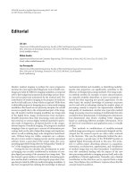
Figure 6: (a) Cameraman and (b) Lena images degraded by 5 × 5
pill-box blur, BSNR = 30 dB.

divided into three separate operators:
fk+1 = P f ,pos P f ,fix P f ,update G fk ,

(26)

where P f ,pos is the positivity operator, P f ,fix denotes the projection onto the bounds which are not updated from fk ,
P f ,update denotes the projection onto the updated bounds,
and G(·) is the steepest descent operator. The indices of
the constraints fixed at iteration k form the set ᏿fix , and
the indices of the updated constraints form ᏿update , where
᏿fix ∩ ᏿update = ∅.
Let the combined mapping P f ,update G be denoted by T.

Then
fk+1 − fk = P f ,pos P f ,fix T fk − P f ,pos P f ,fix T fk−1
≤ P f ,fix T fk − P f ,fix T fk−1

(27)

≤ T f k − T f k −1

because the projections P f ,pos and P f ,fix do not change between iterations k and k − 1, and any projection is, by definition, nonexpansive, that is, for f1 , f2 ∈ Ᏼ, Pf1 − Pf2 ≤
f1 − f2 .


h(m, n)

Spatially Adaptive Intensity Bounds for Image Restoration

1175

0.09
0.08
0.07
0.06
0.05
0.04
0.03
0.02
0.01
0
5
4

3
2

m

1 1

2

4

3

5

n

(b) Estimated blur: ∆h = 0.15.

(a) Restored image: ISNR = 3.73 dB.

0.05

h(m, n)

0.04
0.03
0.02
0.01
0

5
4
3
2

m

1 1
(d) Estimated blur: ∆h =

(c) Restored image: ISNR = 6.39 dB.

2

4

3

5

n

8.0 × 10−16 .

Figure 7: Restoration of Figure 6a with (a), (b) uniform regularisation only (α = 0.09): 204 image updates in 17 cycles; (c), (d) updated
bounds (β = 30, α = 0.05): 748 image iterations in 20 cycles.

The nonlinear operator T is linearised by means of the
Jacobian matrix JT :
T fk − T fk−1 ≈ JT fk fk − fk−1 .


(28)

The (m, n)th element of the Jacobian JT is given by
∂Tm f
JT mn =
,
∂ fn

In this case, m corresponds to a pixel at which the bounds are
fixed between iterations k − 1 and k, or the iterate lies within
the updated bounds. Therefore, Tm represents the steepest
descent step
Tm f = Gm f
= f (m) + µg(m) ∗ h(−m)

(29)

− µ h(m) ∗ h(−m) + αc(m) ∗ c(−m) ∗ f (m),

(31)

where Tm is the mth element of the vector T(f) and fn is the
nth element of the vector f.
The matrix JT is derived by dividing the pixels into three
sets which represent the possible outcomes at each iteration.
(1) The first set is

and hence,
JT


mn

= δ(m − n)
− µ h(m − n) ∗ h(n − m)

+ αc(m − n) ∗ c(n − m) ,

᏿grad = ᏿fix ∪ m ∈ ᏿update :
M f (m) − βσ 2 (m) ≤ Gm (f) ≤ M f (m)+βσ 2 (m) .
f
f
(30)

m ∈ ᏿grad .
(32)

(2) The second set is
᏿high = {m ∈ ᏿update : Gm (f) > M f (m) + βσ 2 (m)}.
f

(33)


EURASIP Journal on Applied Signal Processing

h(m, n)

1176


0.09
0.08
0.07
0.06
0.05
0.04
0.03
0.02
0.01
0
5
4
3
2

m

1

1

2

3

4

5

n


(b) Estimated blur: ∆h = 0.24.

(a) Restored image: ISNR = 3.18 dB.

0.05

h(m, n)

0.04
0.03
0.02
0.01
0
5
4
3
2

m

1

1

2

3

4


5

n

(d) Estimated blur: ∆h = 4.7 × 10−4 .

(c) Restored image: ISNR = 5.38 dB.

Figure 8: Restoration of Figure 6b with (a), (b) uniform regularisation only (α = 0.12): 172 image updates in 17 cycles; (c), (d) updated
bounds (β = 30, α = 0.05): 978 image iterations in 20 cycles.

The steepest descent iterate lies above the upper bound,
which has been updated from the previous image estimate.
The operator Tm becomes
Tm f = M f (m) + βσ 2 (m)
f
1
=
Λ r ∈᏿
+ β

f (r)

win (m)

=






Λ

0,

n ∈ ᏿win (m),
n ∈ ᏿win (m).
/
(35)

᏿low = m ∈ ᏿update : Gm (f) < M f (m) − βσ 2 (m) .
f



Λ r ∈᏿

mn

(3) The third set is

win (m)


1

JT



1


1 + 2β f (n) − M f (m) ,

1
f (r) −
Λ r ∈᏿
2

win (m)

f (r)

2



,

The steepest descent iterate lies below the lower bound, and
therefore, for m ∈ ᏿low ,

(34)
where ᏿win (m) denotes the window of Λ pixels over which
the local statistics at the mth pixel are measured. Then, for
m ∈ ᏿update

(36)


JT

mn

=


1


1 − 2β f (n) − M f (m) ,

Λ



0,

n ∈ ᏿win (m),
n ∈ ᏿win (m).
/
(37)


Spatially Adaptive Intensity Bounds for Image Restoration
Since
T fk − T fk−1

≈ JT fk
≤ JT fk


fk − fk−1
· fk − fk−1 ,

(38)

a sufficient (but not necessary) condition for convergence is
JT (fk ) < 1, k = 1, 2, . . . , ∞, where · represents the L2
norm [25]. While this condition cannot be satisfied for all
possible fk , some observations can be made about the typical
behaviour of the bound update schemes when the degraded
image is used to initialise the iteration.
Assuming that most pixels belong to ᏿grad , that is, the
bounds have not been updated from fk or the iterate falls
within the updated bounds, the matrix JT will have the predominant form of the block-circulant matrix I − µ(H T H +
αC T C). The L2 norm of this matrix is maxm |1 − µλm |, where
λm denotes an eigenvalue of H T H + αC T C. The desired norm
θ < 1 can be obtained if there exists a µ which satisfies
1−θ
1+θ
<µ<
.
λmin
λmax

that the blur estimate h belongs to the Hilbert space Ᏼ defined previously. Like the image, the estimated blur coefficients are constrained to be nonnegative, that is, h(m, n) ≥ 0,
(m, n) ∈ Ω. It is further assumed that the blurring process
preserves energy, and therefore, (m,n)∈Ω h(m, n) = 1 [26,
page 69].
Typically, the blur is negligible outside a small region of

support ᏿h which is not known precisely. Therefore, a conservatively large support is used to initialise the blur estimate.
At the end of each blur optimisation, the estimated support
is pruned such that a rectangular support is maintained. In
truncating the support, an estimate h(m, n) on a row/column
bordering the PSF is assumed to be negligible if it is an order
of magnitude smaller than its nearest neighbour in the adjacent row/column [1, Chapter 6].
Within the estimated support, the PSF is assumed to be
symmetric [27], that is,
h(m, n) = h(−m, −n),

(40)

(39)

The rows belonging to ᏿high or ᏿low have the structure
of the pill-box blur convolution matrix, with additive zeromean fluctuations. These fluctuations are small because the
bounds are activated in the regions of relatively low variance.
Therefore, the norm of a matrix formed from a combination
of these rows will be approximately 1, closely corresponding
to the all-one eigenvector.
The pixels in ᏿high , ᏿low , or ᏿grad are usually clustered
together in regions whose dimensions greatly exceed those of
the window used to calculate the local statistics. Thus, JT can
be partitioned into nearly block-circulant submatrices corresponding to neighbouring pixels in either sets. Because the
nonzero elements of the submatrices correspond to a small
window around the current pixel m, they do not overlap
significantly column-wise or row-wise, and the norm of JT
can be approximated by the largest norm of the submatrices.
From the previous discussion, this is close to 1 if µ satisfies
(39). Simulations indicate that small violations of the convergence condition JT < 1 are partially compensated by

the operators Ppos and Pfix .
5.

1177

BLIND IMAGE RESTORATION

In the previous sections, spatially adaptive intensity bounds
were used in nonblind image restoration to limit noise amplification due to the ill-conditioning of the blur matrix. In
this section, the intensity bounds are applied to blind image restoration in order to further define the solution and to
reduce noise. An alternating minimisation approach, which
switches between constrained optimisation of the image and
the blur, is used. This approach has the advantage that the
methods described in Section 4 can easily be extended to
blind image restoration.
5.1. Characterisation of the blur
The constraints on the blur presented in this section are intended to describe a large class of degradations. It is assumed

where h(−m, −n)
h(Lm − m, Ln − n), and the image is
of dimension Lm × Ln . In this case, the phase of the discrete
Fourier transform of the blur is either 0 or ±π.
Experience indicates that it is necessary to impose
smoothness constraints on the blur itself. Previously, this was
done in the form of a second regularisation term via an extension of either the constrained least squares approach [23]
or the total variation method [28]. The disadvantage of this
method is that the knowledge of the blur support is implicitly needed to determine the blur regularisation parameter [28]. Therefore, an alternative monotonicity constraint
is proposed, which states that the blur should be nonincreasing in the direction of the positive blur axes. This constraint
describes many common blurs, such as the pill-box blur and
the Gaussian blur, and is expressed mathematically as

h(m + 1, n) ≥ h(m, n),

m ≥ 0, (m + 1, n) ∈ ᏿h ,

h(m, n + 1) ≥ h(m, n),

n ≥ 0, (m, n + 1) ∈ ᏿h .

(41)

The monotonicity constraint is extended to the entire support by means of the symmetry constraint.
5.2. Alternating minimisation approach
The proposed alternating minimisation algorithm follows
the general framework of projection-based blind deconvolution [6] but differs in the procedure used to optimise the blur.
In contrast to the algorithms proposed in [23, 28], the constraints are incorporated directly in the optimisation rather
than applied at the end of each minimisation with respect to
either the image or the blur.
Since both f and h are unknown, the cost function becomes
J f, h = g − f ∗ h

2

2

+ α Cf .

(42)

Equation (42) is convex with respect to either f or h, but
not jointly convex. Therefore, the cost function is minimised



1178

EURASIP Journal on Applied Signal Processing

most easily by fixing one estimate and optimising with respect to the other. The roles are then reversed and the process
is repeated until the algorithm converges to a local minimum
[6].
Since the spatially adaptive intensity bounds have a welldefined projection operator, the image optimisation step is
implemented using the constrained steepest descent algorithm (gradient projection method) described in [5]. The
advantage of this method is its simplicity and ease of implementation. The introduction of intensity bounds increases
the linear convergence rate of the steepest descent algorithm
because the bounds impose tight constraints on the solution
[29, 30]. Furthermore, the degraded image provides a good
initial estimate of the original image.
The intensity bounds are reinitialised according to (21),
at the beginning of each image optimisation. During the
minimisation cycle, they are applied as the variance estimates
converge.
For the blur optimisation, the slow convergence rate of
the gradient projection method poses a severe problem since
the blur may be initialised far from the actual solution. Furthermore, an explicit expression for the projection operator
Ph is not readily available as Ꮿh is defined by the intersection
of several convex sets which are not easily combined.
The structure of the blur optimisation problem is better suited to quadratic programming (QP) because (42) is
quadratic with respect to h, subject to the linear equality and
inequality constraints described in Section 5.1. (A good description of QP can be found in [31].) The assumed support
of the blur is usually quite small relative to the image, and so
the QP algorithm can easily handle the number of variables.

The resulting blind image restoration algorithm is described below.
(1) Choose a conservatively large estimate for the PSF support −Nm ≤ m ≤ Nm and −Nn ≤ n ≤ Nn . Initialise the
image and blur estimates to (f0 , h0 ) = (P f g, e1 ), where
e1 denotes the unit vector corresponding to the twodimensional δ-function. Set the cycle number k = 1.
(2) Minimise with respect to the blur using the QP algorithm to obtain hk = arg{minh∈Ꮿh J(fk−1 , h)}.
(3) Truncate the estimated PSF support according to the
following conditions.
(i) If Nm > 0 and h(Nm , n) ≤ 0.1h(Nm − 1, n), −Nn
≤ n ≤ Nn , then Nm = Nm − 1.
(ii) If Nn > 0 and h(m, Nn ) ≤ 0.1h(m, Nn − 1), −Nm
≤ m ≤ Nm , then Nn = Nn − 1.
(iii) Renormalise the truncated blur.
(4) Minimise with respect to the image to obtain fk =
0
arg{min f ∈Ꮿ f J(f, hk )}. Set fk = fk−1 and initialise the
intensity bounds according to (21). Iterate
n+1
n
n
T
fk = P n P n−1 · · · P 0 I − αµC T C fk + µHk g − Hk fk ,
f f
f
(43)

where Hk is a block-Toeplitz matrix of the shifted blur
vectors and the step size µ satisfies (16). The projections P rf , r = 0, . . . , n, are defined in a manner similar

to (25) with k → n. Terminate when
n+1

n
fk − fk
n
fk

2

2

≤δ

(44)

or n > 100.
(5) Repeat steps (2), (3), and (4) until
fk+1 , hk+1 − fk , hk
2
f k , hk

2

≤δ

(45)

or k > 20.
5.3.

Experimental results


The Cameraman and Lena images, superimposed on a black
background, were degraded by a 5 × 5 pill-box blur with
30 dB noise, as shown in Figures 6a and 6b.
A uniform smoothness constraint was used in conjunction with the intensity bounds. A moderate value of α1 =
0.05 was chosen for the regularisation parameter. The scaling
parameter β = 30 was found to give good restorations, but
no attempt was made to fine-tune this value. For comparison, the images were restored using uniform regularisation
only. In this case, the suggested value of α = g −Hf 2 / Cf 2
was used [22], even though these quantities are not usually
known precisely.
The image and blur estimates are shown in Figures 7 and
8. The ISNR was calculated over the image support only. The
quality of the blur estimate was measured as follows:

∆h =

(m,n)∈᏿h ∪᏿h

h(m, n) − h(m, n)

(m,n)∈᏿h ∪᏿h

h(m, n)

2

2

.


(46)

It can be seen that the addition of intensity constraints
significantly improved both estimates. Furthermore, the blur
estimate is very precise due to the proper application of
constraints such as positivity, energy preservation, circular
symmetry, and monotonicity. In particular, the monotonicity constraint, which has not been used in previous blind
restoration schemes, significantly improves the blur estimate.
The main drawback of the bound update algorithm was the
increase in the number of iterations required for the image
optimisation. This can be seen by comparing the number of
image updates for fixed bounds and updated bounds in Figures 7 and 8.
6.

DISCUSSION AND CONCLUSIONS

This paper presented a new method of defining and incorporating spatially adaptive intensity bounds in both blind
and nonblind image restoration. The intensity bounds were
initially estimated from the local statistics of the degraded
image and were updated from the current image estimate
to produce more accurate constraints. It was found that if
the bound scaling parameter β was chosen properly, then
the addition of intensity bounds significantly improved the


Spatially Adaptive Intensity Bounds for Image Restoration
restoration, with the largest improvement resulting from the
proposed bound-update methods. General guidelines for the
choice of the scaling parameter were presented.
While the intensity bounds were implemented in the

context of the gradient projection method, a number of blind
restoration algorithms could be easily modified to incorporate the bounds. Further research needs to be done on the
effectiveness of the intensity bounds in these algorithms.
REFERENCES
[1] A. K. Katsaggelos, Ed., Digital Image Restoration, SpringerVerlag, Berlin, Germany, 1991.
[2] D. Kundur and D. Hatzinakos, “Blind image deconvolution,”
IEEE Signal Processing Magazine, vol. 13, no. 3, pp. 43–64,
1996.
[3] A. N. Tikhonov and V. Y. Arsenin, Solutions of Ill-Posed Problems, John Wiley & Sons, NY, USA, 1977.
[4] D. Kundur and D. Hatzinakos, “A novel blind deconvolution
scheme for image restoration using recursive filtering,” IEEE
Trans. Signal Processing, vol. 46, no. 2, pp. 375–390, 1998.
[5] R. L. Lagendijk, J. Biemond, and D. E. Boekee, “Regularized iterative image restoration with ringing reduction,” IEEE
Trans. Acoustics, Speech, and Signal Processing, vol. 36, no. 12,
pp. 1874–1888, 1988.
[6] Y. Yang, N. P. Galatsanos, and H. Stark, “Projection-based
blind deconvolution,” Journal of the Optical Society of America,
vol. 11, no. 9, pp. 2401–2409, 1994.
[7] M. I. Sezan and A. M. Tekalp, “Adaptive image restoration
with artifact suppression using the theory of convex projections,” IEEE Trans. Acoustics, Speech, and Signal Processing,
vol. 38, no. 1, pp. 181–185, 1990.
[8] S.-S. Kuo and R. J. Mammone, “Image restoration by convex
projections using adaptive constraints and the L1 norm,” IEEE
Trans. Signal Processing, vol. 40, no. 1, pp. 159168, 1992.
[9] S. Kaczmarz, Angenă herte Auă sung von Systemen linearer
a
o
Gleichungen, Bull. Acad. Polon. Sci., vol. A35, pp. 355–357,
1937.
[10] M. C. Hong, T. Stathaki, and A. K. Katsaggelos, “Iterative

regularized image restoration using local constraints,” in
Proc. IEEE Workshop on Nonlinear Signal and Image Processing, Mackinac Island, Mich, USA, September 1997.
[11] M. G. Kang and A. K. Katsaggelos, “General choice of the regularization functional in regularized image restoration,” IEEE
Trans. Image Processing, vol. 4, no. 5, pp. 594–602, 1995.
[12] A. K. Katsaggelos and M. G. Kang, “Spatially adaptive iterative
algorithm for the restoration of astronomical images,” International Journal of Imaging Systems and Technology, vol. 6, no.
4, pp. 305–313, 1995.
[13] K. May, T. Stathaki, and A. K. Katsaggelos, “Iterative blind
image restoration using local constraints,” in Proc. European
Conference on Signal Processing, pp. 335–338, Rhodes, Greece,
September 1998.
[14] K. May, T. Stathaki, and A. K. Katsaggelos, “Blind image
restoration using local bound constraints,” in Proc. IEEE
Int. Conf. Acoustics, Speech, Signal Processing, vol. 5, pp. 2929–
2932, Seattle, Wash, USA, May 1998.
[15] K. May, T. Stathaki, A. G. Constantinides, and A. K. Katsaggelos, “Iterative determination of local bound constraints in iterative image restoration,” in Proc. IEEE International Conference on Image Processing, vol. 2, pp. 833–837, Chicago, Ill,
USA, October 1998.
[16] K. Miller, “Least squares methods for ill-posed problems with
a prescribed bound,” SIAM Journal on Mathematical Analysis,
vol. 1, pp. 52–74, 1970.

1179
[17] G. L. Anderson and A. N. Netravali, “Image restoration based
on a subjective criterion,” IEEE Trans. Systems, Man, and Cybernetics, vol. 6, no. 12, pp. 845–853, 1976.
[18] A. K. Katsaggelos, “A general formulation of adaptive iterative
image restoration algorithms,” in Proc. IEEE Conference on
Information Sciences and Systems, pp. 42–47, Princeton, NJ,
USA, March 1986.
[19] A. K. Katsaggelos, J. Biemond, R. M. Mersereau, and R. W.
Schafer, “Non-stationary iterative image restoration,” in

Proc. IEEE Int. Conf. Acoustics, Speech, Signal Processing, vol. 2,
pp. 696–699, Tampa, Fla, USA, March 1985.
[20] W.-J. Song and W. A. Pearlman, “Edge-preserving noise filtering based on adaptive windowing,” IEEE Trans. Circuits and
Systems, vol. 35, no. 8, pp. 1048–1055, 1988.
[21] S. N. Efstratiadis and A. K. Katsaggelos, “Adaptive iterative
image restoration with reduced computational load,” Optical
Engineering, vol. 29, no. 12, pp. 1458–1468, 1990.
[22] A. K. Katsaggelos, J. Biemond, R. W. Schafer, and R. M.
Mersereau, “A regularized iterative image restoration algorithm,” IEEE Trans. Signal Processing, vol. 39, no. 4, pp. 914–
929, 1991.
[23] Y.-L. You and M. Kaveh, “A regularization approach to joint
blur identification and image restoration,” IEEE Trans. Image
Processing, vol. 5, no. 3, pp. 416–428, 1996.
[24] A. K. Katsaggelos, “Iterative image restoration algorithms,”
Optical Engineering, vol. 28, no. 7, pp. 735–748, 1989.
[25] R. W. Schafer, R. M. Mersereau, and M. A. Richards, “Constrained iterative restoration algorithms,” Proceedings of the
IEEE, vol. 69, no. 4, pp. 432–450, 1981.
[26] H. C. Andrews and B. R. Hunt, Digital Image Restoration,
Prentice-Hall, Englewood Cliffs, NJ, USA, 1977.
[27] A. M. Tekalp, H. Kaufman, and J. W. Woods, “Identification
of image and blur parameters for the restoration of noncausal
blurs,” IEEE Trans. Acoustics, Speech, and Signal Processing,
vol. 34, no. 4, pp. 963–972, 1986.
[28] T. F. Chan and C.-K. Wong, “Total variation blind deconvolution,” IEEE Trans. Image Processing, vol. 7, no. 3, pp. 370–375,
1998.
[29] R. L. Lagendijk, R. M. Mersereau, and J. Biemond, “On increasing the convergence rate of regularized iterative image
restoration algorithms,” in Proc. IEEE Int. Conf. Acoustics,
Speech, Signal Processing, vol. 2, pp. 1183–1186, Dallas, Tex,
USA, April 1987.
[30] A. K. Katsaggelos and S. N. Efstratiadis, “A class of iterative

signal restoration algorithms,” IEEE Trans. Acoustics, Speech,
and Signal Processing, vol. 38, no. 5, pp. 778–786, 1990.
[31] R. Fletcher, Practical Methods of Optimisation, John Wiley &
Sons, Chichester, West Sussex, UK, 2nd edition, 1987.
Kaaren L. May was born in London,
Canada, in 1973. After completing her
B.S.E. in engineering physics in 1995 at
Queen’s University, Kingston, Canada, she
won a Commonwealth scholarship to study
for a Ph.D. in signal processing at Imperial College of Science, Technology, and
Medicine in London, England. She was
awarded the Ph.D. degree in 1999 and spent
the following year working for the Defence
Evaluation and Research Agency (DERA) as a Postdoctoral Research Associate at Imperial College. She joined the broadcast manufacturer Snell and Wilcox in 2000, and currently works as a Senior Research Engineer at their Research Centre in Liss, Hampshire.
Her research interests include image restoration, motion estimation, and nonlinear modelling.


1180
Tania Stathaki was born in Athens, Greece.
In September 1991, she received the M.S.
degree in electronics and computer engineering from the Department of Electrical
and Computer Engineering of the National
Technical University of Athens (NTUA) and
the Advanced Diploma in Classical Piano
Performance from the Orfeion Athens College of Music. She received the Ph.D. degree
in signal processing from Imperial College
in 1994. Since 1998 she has been a Lecturer in the Department of
Electrical and Electronic Engineering at Imperial College and the
Image Processing Group Leader of the same department. Previously, she was a Lecturer in the Department of Information Systems and Computing at Brunel University in the UK and a Visiting
Lecturer in the Electrical Engineering Department at Mahanakorn

University in Thailand. Her current research interests lie in the areas of image processing, nonlinear signal processing, signal modelling, and biomedical engineering. Dr. Stathaki is the Author of 70
journal and conference papers. She has been, and is currently serving as, a member of many technical program committees of the
IEEE, the IEE, and other international conferences. She also serves
as a member of the editorial board of several professional journals.
Aggelos K. Katsaggelos received the
Diploma degree in electrical and mechanical engineering from the Aristotelian
University of Thessaloniki, Greece, in
1979, and the M.S. and Ph.D. degrees,
both in electrical engineering, from the
Georgia Institute of Technology, in 1981
and 1985, respectively. In 1985, he joined
the Department of Electrical and Computer
Engineering at Northwestern University,
where he is currently Professor, holding the Ameritech Chair of
Information Technology. He is also the Director of the Motorola
Center for Communications and a member of the Academic
Affiliate Staff, Department of Medicine, at Evanston Hospital.
Dr. Katsaggelos is a member of the publication board of the
IEEE Proceedings, the IEEE Technical Committees on Visual
Signal Processing and Communications, and Multimedia Signal
Processing, Marcel Dekker: Signal Processing Series, Applied
Signal Processing, and Computer Journal. He has served as Editorin-Chief of the IEEE Signal Processing Magazine (1997–2002), a
member of the Board of Governors of the IEEE Signal Processing
Society (1999–2001), and a member of numerous committees.
He is the Editor of Digital Image Restoration (Springer-Verlag,
1991), Coauthor of Rate-Distortion Based Video Compression
(Kluwer, 1997), and Coeditor of Recovery Techniques for Image
and Video Compression and Transmission (Kluwer, 1998). He is
the coinventor of eight international patents, a fellow of the IEEE,
and the recipient of the IEEE Third Millennium Medal (2000), the

IEEE Signal Processing Society Meritorious Service Award (2001),
and an IEEE Signal Processing Society Best Paper Award (2001).

EURASIP Journal on Applied Signal Processing