Hindawi Publishing Corporation
EURASIP Journal on Advances in Signal Processing
Volume 2007, Article ID 37485, 20 pages
doi:10.1155/2007/37485
Research Article
Tracking Signal Subspace Invariance for Blind Separation and
Classification of Nonorthogonal Sources in Correlated Noise
Karim G. Oweiss
1
and David J. Anderson
2
1
Electrical & Computer Engineer ing Department, Michigan State University, East Lansing, MI 48824-1226, USA
2
Electrical Engineering & Computer Science Department, University of Michigan, Ann Arbor, MI 48109-2122, USA
Received 1 October 2005; Revised 11 April 2006; Accepted 27 May 2006
Recommended by George Moustakides
We investigate a new approach for the problem of source separation in correlated multichannel signal and noise environments.
The framework targets the specific case when nonstationary correlated signal sources contaminated by additive correlated noise
impinge on an array of sensors. Existing techniques targeting this problem usually assume signal sources to be independent, and
the contaminating noise to be spatially and temporally white, thus enabling orthogonal signal and noise subspaces to be separated
using conventional eigendecomposition. In our context, we propose a solution to the problem when the sources are nonorthog-
onal, and the noise is correlated with an unknown temporal and spatial covariance. The approach is based on projecting the
observations onto a nested set of multiresolution spaces prior to eigendecomposition. An inherent invariance property of the sig-
nal subspace is observed in a subset of the multiresolution spaces that depends on the degree of approximation expressed by the
orthogonal basis. This feature, among others revealed by the algorithm, is eventually used to separate the signal sources in the
context of “best basis” selection. The technique shows robustness to source nonstationarities as well as anisotropic properties of
the unknown signal propagation medium under no constraints on the array design, and with minimal assumptions about the
underlying signal and noise processes. We illustrate the high performance of the technique on simulated and experimental multi-
channel neurophysiological data measurements.
Copyright © 2007 K. G. Oweiss and D. J. Anderson. This is an open access article distributed under the Creative Commons

Attribution License, which permits unrestricted use, distribution, and reproduction in any medium, provided the original work is
properly cited.
1. INTRODUCTION
Multichannel signal processing aims at fusing data collected
at several sensors in order to carry out an estimation task
of signal sources. Generally speaking, the parameters to be
estimated reveal important information characterizing the
sources from which the data is observed. The aim of array
signal processing is to extract these parameters with the min-
imal deg ree of uncertaint y to enable detection and classifi-
cation of these sources to take place. Many ar ray signal pro-
cessing algorithms rely on eigenstructure subspace methods
performed either in the time domain, in the frequency do-
main, or in the composite time-frequency domain [1–3]. Re-
gardless of which domain is used, eigenst ructure based al-
gorithms offer an optimal solution to many array processing
applications provided that the model assumptions about the
underlying signal and noise processes are appropriate (e.g.,
independent source signals, uncorrelated signals and noise,
spatially and temporally white noise processes, etc.) [4–7].
For some applications, many of these assumptions can-
not be intrinsically made, such that when the sources
have correlated waveform shapes and the noise is corre-
lated among sensors, or when the propagating medium is
anisotropic. Many approaches have been suggested in the
literature to mitigate the effects of unknown spatially cor-
related noise fields to enable better source separation of
the array mixtures and showed various degrees of suc-
cess (see [6–8] and the references therein). Nevertheless,
the particular case where signal sources are nonorthogonal

and may inherently possess considerable correlation with
the contaminating noise has not received considerable at-
tention. This situation may occur, for example, when the
noise is the result of the presence of a large number of
weak sources that generate signal waveforms identical to
those of the desired ones. Recording of neuronal ensem-
bles in the brain with microelectrode arrays is a classi-
cal example where such situation is frequently encountered
[9, 10].
2 EURASIP Journal on Advances in Signal Processing
The objective of this paper is to develop a new technique
for separating and potentially classifying a number of corre-
lated sources impinging on an array of sensors in the pres-
ence of strong correlated noise. Although we focus specifi-
cally on neural signals recorded by microelectrode arrays in
the nervous system as the primary application, the technique
is applicable to a wide variety of applications where simi-
lar signal and noise characteristics are encountered. The pa-
per targets the source separation problem in detail, while the
classification task using the features obtained is detailed else-
where [11]. In that respect, we make the following assump-
tions about the problem at hand.
(1) T he observations are an instantaneous mixture of
w ide-band signals.
(2) Sources are not in the far field, are nonorthogonal with
signals that are transient-like, and may be fully or par-
tially coherent across the array.
(3) The number of sources within the analysis interval is
unknown.
(4) Thenoiseisamixtureoftwocomponents:

(a) zero mean independent, identically distributed
(iid) Gaussian white noise (e.g., thermal and electronic
noise),
(b) correlated noise component with unknown tem-
poral and spatial covariance resulting from numerous
interfering weak sources.
The technique proposed exploits mainly spatial diversity
in the signals observed under the assumptions stated above
[12]. It does not attempt to exploit delay spread or frequency
spread [13]. In that regard, we focus on the blind separa-
tion of the sources without trying to identify the channel.
Though our model is the classical linear array model typi-
cally used in array processing literature, it does not assume a
linear time invariant (LTI) finite impulse response (FIR) sys-
tem to model the channel, as is the case in typical multiple-
input multiple-output (MIMO) systems [13, 14]. Because of
the existence of the sources in the proximity of the array, and
the fact that the signal sources cannot be treated as point
sources
1
as we will demonstrate later, classical direction of
arrival (DOA) techniques are generally inapplicable.
The paper is organized as follows: Section 2 describes rel-
evant array processing theory starting from the signal model
in the absence of noise and in the presence of noise. Section 3
describes the advantages gained by orthogonal t ransforma-
tion prior to eigendecomposition. The formulation of the al-
gorithm is detailed by analyzing the array model in the mul-
tiresolution domain. In Section 4, we demonstrate the per-
formance of the algorithm using simulated and experimental

data.
To clarify the notation, we will adhere to the somewhat
standard notation convention. Uppercase, boldface charac-
ters will generally refer to random matrices, while uppercase,
boldface nonitalic characters will generally refer to deter-
1
In neurophysiological recording, every element of the signal source (neu-
ron) is capable of generating a signal and therefore the signal source can-
not be regarded as a point source [15].
ministic matrices (e.g., linear transformations). Lowercased
boldfaced characters will generally refer to column vectors.
Eigenvalues of square Hermitian matrices are assumed to be
ordered in decreasing magnitude, as are the singular values
of nonsquare matrices. The notation (
·)
j
will generally refer
to a quantity estimated in the jth frequency subband, except
for correlation matrices, where the notation (
·)
j
Q
will be used
to define the correlation of the Q data matrix estimated in
the jth frequency subband.
2. MATHEMATICAL PRELIMINARIES
Consider a model of P signals impinging on an array of M
sensors expressed in terms of the M
× 1 signal vector over an
observation interval of length N:

x(n)
= As(n), n = 0, , N − 1, (1)
where A
∈ R
M×P
denotes the mixing matrix that expresses
the array response to the nth snapshot of P sources s(n)
=
[
s
1
(n) s
2
(n) ··· s
p
(n)
]
T
,whereP ≤ M. Over the observa-
tion interval, each source s
p
is assumed Gaussian distributed
with zero mean and variance σ
2
s
p
, p = 1, , P. The model
can be more conveniently expressed in matrix form as
X
=


x(0) x(1) ··· x(N − 1)

=
AS. (2)
This model is w idely recognized in the arr ay processing com-
munity when it is required to estimate the unknown source
matrix S or their DOAs from an estimate of A. Alternatively,
it is also used in MIMO systems in which a known source
matrix S (training signals) is used to probe the transmission
channel in order to estimate the unknown channel matrix.
In our context, it is assumed that neither A nor S is known.
This situation may occur, for example, in blind source sepa-
ration problems where it is necessary to extract as many sig-
nals as possible from the observed data. The mixing matrix
in this case models three elements: (1) the spatial extent of
the source, (2) the transmission channel that characterizes
the unknown signal propagation medium, and (3) the sen-
sor point spread function [16].
Characterizing the unknown sources has been widely ex-
ploited using second-order statistics of the data matrix. First,
we briefly review some known concepts using vector space
theory. In model (2), the column space of the signal matrix
X is spanned by all the linearly independent columns of A ,
while the row space of X is spanned by the rows of S. Using
second-order statistics, the signal subspace, denoted
{A},can
be identified using singular value decomposition (SVD) as
X
= U

X
D
X
V
T
X
. (3)
When the sources are uncorrelated with unequal energy, then
R
S
= E[SS
T
] = diag[σ
2
S
1
, σ
2
S
2
, , σ
2
S
P
]. The largest P eigen-
values of R
X
= E[XX
T
] are nonzero and correspond to

eigenvectors U
S
= [u
1
, u
2
, , u
P
] ∈ R
M×P
that span the
subspace
{A} spanned by the columns of A. The remaining
M
− P eigenvalues a re zero with probability one, and the re-
maining eigenvectors [u
P+1
, u
P+2
, , u
M
] span the null space
K. G. Oweiss and D. J. Anderson 3
of A. This analysis is guaranteed to separate the sources from
knowledge of A, or a least squares (LS) estimate of A [4].
When the source signals are nonorthogonal, that is,
s
i
, s
j

 = 0, where · denotesadotproduct,R
S
has an
(i, j)th entry given by
R
S
(i, j) = ρ
ij
σ
s
i
σ
s
j
=
P

p=1
λ
p
u
p
[i]u
T
p
[ j], (4)
where ρ
ij
expresses the unknown correlation between the ith
and jth sources. Therefore, each eigenvalue λ

p
corresponds
to the mixture of sources that have nonzero projection along
the direction of eigenvector u
p
. Therefore, the strength of the
ith mode of the signal covariance can be expressed as
λ
i
= σ
s
i
P

i=1
ρ
ij
σ
s
j
, i = 1, , P. (5)
This results in an ambiguity in identifying the signal sub-
space. This occurs because each eigenvector spans a direction
determined by the correlated component of the sources and
not that of each individual source.
3. ORTHOGONAL TRANSFORMATION
3.1. Noise-free model
Our approach for solving this complex problem relies on
exploiting an alternative solution to signal subspace deter-
mination. Recall from (4) that the signal subspace is a P-

dimensional space that can be determined from the span of
the columns of A. Alternatively, it can be determined from
the P rows of S if signal correlation is minimized by appro-
priate signal subspace rotation. If the rotation does not alter
the span of the columns of A, then it can be used to sep-
arate the correlated sources. This can be seen if the mixing
matrix is decomposed as A
= QH
T
[17]. The M × P ma-
trix Q corresponds to a whitening matrix that can be de-
termined from the data if training sequences are available.
On the other hand, H is a P
× P unitary rotation matrix on
the space
R
P×1
.In[17], a semiblind MIMO approach was
suggested to determine Q and H from the pilot data (train-
ing sequence). However in the current problem, we stress the
notion that the purpose is to blindly separate and classify P
unknown sources, and not to estimate the channel. Even if
samples of the source signals are available for t raining after
an initial signal extraction phase for example, they will not
fulfill the orthogonality condition typically required in pilot
signals. Because A can be expressed using SVD as A
= EΣΓ
T
,
then a suggested choice [17]forQ would be Q

= EΣ, while
H
= Γ. However, this factorization assumes that A is known.
Note that the M
×P matrix of eigenvectors U
S
can be utilized
as an alternative to finding Q from unavailable training data.
However, there are two conditions that have to be satisfied in
order to utilize U
S
: (1) the signal sources have to be orthog-
onal with a sufficiently long data stream to avoid biasing the
estimate of Q, and (2) the number of sources P to be sepa-
rated is known to determine the number of columns of U
S
.
Clearly both conditions are inapplicable given the assump-
tions we stated above.
Our alternative approach is to approximately “null” the
effect of the rotation matrix H on the source matrix S. This
can be achieved using a wide range of orthogonal transfor-
mation. The idea is to find a particular orthogonal transfor-
mation to undo the rotation caused by H, or equivalently
minimize signal correlation. For reasons that will become
clear in the sequel, we opted to use an orthogonal basis set
that projects the observation matrix onto a set of nested mul-
tiresolution spaces. This can be efficiently achieved using a
discrete wavelet transformation (DWT) or its overcomplete
version, the discrete wavelet packet transform (DWPT). The

advantage of using the DWPT is the considerable sparseness
it introduces in the transform domain. Besides, the DWPT
orthogonal transformation is known to universally approxi-
mate a wide variety of unknown signals. Taken together, both
properties will allow source separation to take place without
having to estimate the matrix H.
LetusdenotebyW
( j)
an N ×N DWPT orthogonal trans-
formation operator at resolution j,where j
= 0,1, , J.Let
us operate on the data matrix in (2), so we obtain
X
j
= AS W
( j)
= AS
j
, j = 0, 1, , J,(6)
where S
j
denotes the source matrix projected onto the space
Ω
j
of all piecewise smooth functions in L
2
(R). These are
spanned by the integer-translated and dilated copies φ
j,k
def

=
2
j/2
φ(2
j
·
− k) of a scaling function φ that has compact sup-
port [18]. In practice, ( 6) is obtained by performing an un-
decimatedDWPTprojectiononeachrowofX separately and
stacking the results in the M
× N matrix X
j
.Spectralfactor-
ization of (6) using SVD yields
X
j
= U
j
X
D
j
X
V
j
T
X
=
M

i=1

λ
j
i
u
j
i
v
j
T
i
. (7)
The columns of the eigenvector matrix V
j
X
span the row space
of X
j
, that is, the space spanned by the transformed signals
s
j
p
, p = 1, , P, which are now sparse. This means that s
j
p
will have a few entries that are nonzero. The sparsity in-
troduced by the DWPT operator enables us to infer a rela-
tionship between the row space of X
j
and that of X using
the whitening-rotation factorization of A discussed above.

Specifically, if W
( j)
spans the null space of the product H
T
S,
the corresponding rows of H
T
S
j
will be zero. Conversely, if
W
( j)
spans the range space of H
T
S, then the corresponding
rows of H
T
S
j
will be nonzero. Furthermore, they w ill belong
to the subspace spanned by the columns of the whitening ma-
trix Q, or equivalently U
S
.
Given the spectral factorization of X
j
in (7),anecessary
(but not sufficient) condition for a column of V
j
X

to span
the row space of X
j
is the existence of at least one row of
H
T
S
j
that is nonzero with probability one. If such a row exist,
then a corresponding independent column in U
j
X
will exist.
This argument elucidates that any perturbation in the num-
ber of linearly independent columns in V
j
X
, which is directly
4 EURASIP Journal on Advances in Signal Processing
associated with the number of distinct eigenvalues along the
diagonal entries in D
j
X
, will directly impact the correspond-
ing independent columns of U
j
X
. This can be seen from (7)
using the outer product form.
To be more specific, let us denote by Δ

{J} the full dic-
tionary of basis obtained from a DWPT decomposition up
to L decomposition levels
2
(J subbands). Among all the J
bases obtained, a subset of basis is selected from the dictio-
nary Δ
{J} for which W
( j)
spans the range space of H
T
S. This
subset is interpreted as the collection of wavelet basis that
best represent the sources in the range space of H
T
S.Letus
assume that S contains a single source, that is, P
= 1. Let us
denote the subset of basis by J
1
, and the cardinality of the set
J
1
will be denoted J
1
. This implies that there is only J
1
basis
in the DWPT expansion for which h
T

1
s
j
1
, j ∈ J
1
,isnonzero.
Therefore, the signal subspace spanned by the columns of
U
j
X
,denoted{A}
j
, will be restricted to those basis that be-
long to J
1
as evident from (7). We denote the signal subspace
dimension in subband j by P
j
, where it is straightforward to
show that P
j
is always upper bounded by P [19].
Since W
( j)
is arbitrarily chosen and the signals are
nonorthogonal, we expect that in reality there will be mul-
tiple rows in any given subband for which h
T
p

s
j
p
is nonzero,
where h
p
denotes the pth column of H. The goal is there-
fore to rank-order the subbands based on the deg ree to which
they are able to preserve the signal subspace. This is feasible
by rank-ordering the eigenvalues across subbands and exam-
ining their corresponding eigenvectors U
j
X
. Specifically, this
can be achieved in two different ways.
(1) Within subband j, the blind source separation pro-
cess amounts to finding the signal eigenvalues that corre-
spond to the group of sources that possess nonzero projec-
tions onto the jth wavelet basis, that is, h
T
p
s
j
p
is nonzero for
p
= 1, , P
j
. These will be ranked in decreasing order of
magnitude according to

λ
j
1
>λ
j
2
> ··· >λ
j
P
j
⇐⇒ h
T
p
1
s
j
p
1
> h
T
p
2
s
j
p
2
> ··· > h
T
P
j

s
j
P
j
such that p
1
= arg max
p∈{1, ,P
j
}
h
T
p
s
j
p
.
(8)
(2) Given a specific source p
∗
∈{1, , P}, the source
classification process amounts to specifying an operator B
p
∗
,
that finds the set of subband indices among all j
∈ Δ{J} for
which there exist an invariant eigenvector u
j
p

∗
. That is,
λ
j
1
p
>λ
j
2
p
> >λ
J
p
p
>⇐⇒ h
T
p
s
j
1
p
> h
T
p
s
j
2
p
> >h
T

p
s
J
p
p
such that p
∗
= arg min
j∈Δ{J}


u
j
p
∗
− a
p
∗


2
,
(9)
2
For a 2-band orthonormal discrete wavelet packet transform up to L de-
composition levels, a binary tree representation would consist of a total of
J
= 2
L+1
− 1 subbands.

where a
p
∗
denotes the p
∗
th independent column of the ma-
trix A. This set of basis, now labeled J
p
∗
⊂ Δ{J}, will consti-
tute the “best basis” representing the source p
∗
.
3.2. Best basis selection
The second interpretation in (9) f alls under the class of best
basis selection schemes, originally introduced in [20]. The
idea can be summarized as follows. In representing the dis-
crete signal successively into different frequency bands in
terms of a set of overcomplete orthonormal basis functions,
one obtains a dictionary of basis to choose from. These are
represented by a binary tree in which high amplitude wavelet
coefficients in a certain node indicate the presence of the cor-
responding basis in the signal and measure its contribution.
Equivalently, they evaluate the content of the signal inside
the related frequency subband. Best signal representation is
obtained by defining a cost function for pruning the binary
tree. In [20], it was suggested to prune the tree by minimiz-
ing an entropy cost function between the parent and children
nodes. The cost of each node in the binary tree is compared
to the cost of its children. A parent node is marked as a termi-

nal node if it yields a lower cost than its children cost. Other
cost functions such as mean square error (MSE) minimiza-
tion were suggested in [21]. Clearly, one cost function selec-
tion may be suitable for some signal types while not the best
for others.
In our context, the cost function can be expressed in
terms of the invariance property of the signal subspace
{A}
j
of children nodes compared to their parent node. Specifically,
a child node is considered a candidate for further splitting
if the Euclidean distance between the signal subspace in the
parent node and that of the child is minimized. This can be
expressed as
cost(j, p)
= min
j∈J
p


u
j=Parent
p
− u
j=Child
p


2
. (10)

The cost definition ensures that for those children nodes
that do not have a “similar” signal subspace to that of the par-
ent, they will not be marked as candidates for further split-
ting. The search in the binary tree is performed in a top-
down scheme, starting from the time domain signal matrix
Y that is guaranteed to contain the full signal subspace
{A}.
Generally speaking, wavelet coefficients exhibit large inter-
scale dependency [ 22–24]. Therefore, it is anticipated that if
the signal subspace is spanned by the wavelet basis in a parent
node, it will be s panned by the wavelet basis of at least one of
the children nodes.
3.3. Noisy model
Let us now consider the general observation model in the
presence of additive noise. The observation matrix Y
∈
R
M×N
can be expressed as
Y
= X + Z = AS + Z, (11)
where Z
∈ R
M×N
denotes a zero-mean additive noise with
arbitrary spatial and temporal covariances R
Z
∈ R
M×M
and

K. G. Oweiss and D. J. Anderson 5
C
Z
∈ R
N×N
, respectively. Using SVD, Y can be spectr al ly fac-
tored to yield
Y
= U
Y
D
Y
Y
T
V
=
M

m=1
λ
m
u
m
v
T
m
, (12)
where λ
m
denotes the mth singular value corresponding to

the mth diagonal entry in D
Y
= diag[λ
1
···λ
M
], and U
Y
=
[u
1
, u
2
, , u
M
] ∈ R
M×M
comprises the eigenvectors span-
ning the column space of Y, while V
Y
= [v
1
, v
2
, , v
N
]R
N×N
comprises the eigenvectors spanning the row space of Y.IfY
is a linear mixture of P orthogonal signal sources contami-

nated by additive white noise, then the first P columns of U
Y
will span the signal subspace {A}, while the remaining M − P
columns of U
Y
will span the orthogonal noise subspace {Z}.
The matrix Y
j
obtained through orthogonal transforma-
tion W
( j)
can be likewise decomposed using SVD to yield
Y
j
= AS
j
+ Z
j
= U
j
Y
D
j
Y
V
j
T
Y
, (13)
where Z

j
expresses the projection of the noise matrix onto
the subspace Ω
j
. Similar to the analysis in the noise-free case,
the span of V
j
Y
directly impacts the span of the column space
of U
j
Y
.However,thiscaseisnottrivialduetothepresenceof
the noise since the eigenvalues λ
j
P
j
+1
>λ
j
P
j
+2
> ··· >λ
j
M
are
nonzero with probability one.
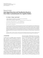
To make the presentation clear, let us consider the sim-
plistic illustration in Figure 1. In this illustration, it is as-

sumed that the dictionary obtained contains a total of three
wavelet basis. For completeness, this implies that all the func-
tions in L
2
(R) reside in the space spanned by the fixed bases
β
i
, β
l
,andβ
k
, respectively. The row space of X = AS,de-
noted
{X}, and the row space of Z,denoted{Z},arepro-
jected onto this three-dimensional wavelet space. This repre-
sentation permits visualizing how the projection of the noise
row space
{Z} results in two components, namely, {Z}
//
that resides in the signal subspace (correlated noise compo-
nent), and
{Z}
⊥
that is orthogonal to the signal subspace
{X} (white noise component). In this representation, {Z}
⊥
is spanned by the wavelet base β
i
. On the other hand, {Z}
//

is spanned by β
l
and β
k
, respectively. The projections of the
noise
{Z}
//
onto these bases are denoted {Z}
l
and {Z}
k
,re-
spectively. In a similar fashion, the signal subspace
{X} can
be projected onto the basis β
l
and β
k
, resulting in the signal
components
{X}
l
and {X}
k
, respectively. It is thus assumed
that β
i
does not represent any of the signal sources, that is,
H

T
S
i
= 0
P×N
. Careful examination of these projections yields
the following.
(1) Any signal projection that belongs to
{X}
l
is dominant
over noise projections
{Z}
l
.
(2) Any noise projection that belongs to
{Z}
k
is dominant
over the signal projections
{X}
k
.
(3) Any noise projection that belongs to
{Z}
⊥
is fully ac-
counted for by the wavelet basis β
i
.

Therefore, the best basis set J
p
for source p would con-
tain only the index l.If
{X} contained only a single source
p, then the dominant eigenvalue λ
l
1
will correspond to the
β
i
Z
i
X
k
Z
k
β
k
Z
//
X
X
l
Z
l
Y
Z
β
l

Figure 1: Projection of the signal and noise subspaces {X} (blue),
and
{Z} (green), respectively, onto a fixed orthogonal basis space.
The space is assumed to be completely spanned by three orthogonal
basis
{β
l
}, {β
k
},and{β
i
} for clarity.
eigenvector u
l
1
spanning the signal subspace, which would be
a 1D space spanned by the single column matrix A.
The sparsity introduced by the orthogonal transforma-
tion again plays an important role in the noisy model. This
is because the noise spreads out across resolution levels to
many small coefficients that are easy to threshold using the
denoising property of the DWT [25, 26]. Therefore, the once
ill-determined separation gap between the signal eigenval-
ues and those of the noise when the noise is caused by weak
sources becomes relatively easier to determine. Thus the ad-
vantages gained by exploiting subspace decomposition in the
transform domain become obvious. These are (1) reduction
of the contribution of the unknown correlation coefficients
ρ
ij

on the eigenvalues of the signal matrix X, and (2) enhanc-
ing the separation gap between the signal and noise eigenval-
ues when the noise is correlated.
3.4. Subband-dependent signal subspace dimension
Generalizing the example in Figure 1 to an ar bitrary number
of wavelet basis in the dictionary obtained, we obtain a set of
wavelet basis β
l
for each source in which the signal subspace
projection
{X}
l
dominates over the noise subspace projec-
tion
{Z}
l
. These are denoted J
1
{l}, J
2
{l}, , J
P
{l}⊂Δ{J}.
3
We reiterate that since both the signal matrix and the mix-
ing matrix are unknown, our interest is to separate the most
dominant sources in the mixture. Due to nonzero correla-
tion among signals, or when P>M, the problem becomes
ill-posed. In that respect, the time domain model in ( 2)may
over/underestimate the dimension of the signal subspace.

However, with the transformed model in (6), the sparsity in-
troduced by the DWPT considerably mitigates the effect of
3
The index l will be used thereafter to indicate the basis indices for which
the signal subspace projection dominates over the noise subspace projec-
tion.
6 EURASIP Journal on Advances in Signal Processing
signal correlation, which maximizes the likelihood of esti-
mating the correct P
j
. We have shown previously [19] that
a multiresolution sphericity test can be used to determine P
j
by examining the ratio of the geometric mean of the eigen-
values, λ
j
m
’s, to the arithmetic mean as
Λ
j
=


M
m
=1
λ
j
m


(1/M−i+1)

1/(M − i +1)


M
m=i
λ
j
m
, i = 1, , M − 1. (14)
This test determines the equality of the smallest eigenval-
ues (presumably the noise eigenvalues), or equivalently how
spherical the noise subspace is. It determines how many sig-
nal subspace components are projected onto the signal sub-
space. The test consists of a series of nested hypothesis tests
[27], testing M
− i eigenvalues for equality. The hypotheses
are of the form
H
0

P
j

: λ
j
1
≥ λ
j

2
≥···λ
j
P
j
+1
= λ
j
P
j
+2
=···=λ
j
M
,
H
1
(P
j
):λ
j
1
≥ λ
j
2
≥···λ
j
P
j
≥ λ

j
P
j
+1
···>λ
j
M
,
i
= 1, , M − 1. (15)
We are interested in finding the smallest value of P
j
for which
the null hypothesis is true. Using a desired performance
threshold for the probability of false alarm (over determina-
tion of P
j
), P
j
dominant modes are described by their corre-
sponding rank ordered P
j
eigenvectors.
We should point out that there are multiple ways the al-
gorithm can be implemented. We summarize below one pos-
sible implementation.
(1) Compute the orthogonal transformation of the obser-
vation matrix row wise up to L decomposition levels.
(2) For each subband, compute the eigendecomposition of
the sample covariance matrix of the transformed ob-

servation matrix.
(3) For each eigenmode, rank-order the subbands based
on the magnitude of their eigenvalues relative to the
0th subband eigenvalue.
(4) For each of the rank-ordered subbands, calculate the
distance between each eigenvector and the corre-
sponding 0th subband eigenvector. If the distances
computed fall below a prespecified threshold, mark
this subband as a candidate node in the best basis tree
J
p
. Otherwise, discard the current node and proceed
to the next rank-ordered subband.
(5) For each of the candidate nodes, proceed in a bottom-
up approach by examining the parent-child relation-
ship between the node indices.
4
Nodes that do not have
a parent node as a member of the candidate nodes set
are discarded from the set J
p
.
4
In a dual-band DWPT tree with linear indexing, a parent node with index
l has children indices 2l +1and2l +2,respectively.
The outcome of these steps will permit identifying the char-
acteristic best basis tree for each of the P sources. This imple-
mentation can be used to interpret the algorithm as a classi-
fier since the signal’s spatial, temporal, and spectral features
are expressed in terms of estimates of the signal parameters

λ
l
p
, u
l
p
for l ∈ J
p
and p = 1, , P. If the sources are Gaussian
distributed, then it can be shown that the estimated parame-
ters are also multivariate nor m al distributed. Therefore they
can be optimally classified using likelihood methods [28, 29].
This analysis is outside the scope of this paper and is reported
elsewhere [11].
3.5. Computational complexity
For the sake of completeness, we discuss briefly the com-
putational complexity of the algorithm. For an M
× N ma-
trix, a full DWPT computation can be done in O(MN)us-
ing classical convolution based algorithms [30]. There are
two ways by which one can reduce this figure. First, the sig-
nals observed are known to be 1st level lowpass, therefore
restricting the initial DWPT tree structure to descendants of
the first level lowpass expansion does not affect the perfor-
mance, but reduces the DWPT computations by 50%. Sec-
ond,wehaveexperiencedwithmoreefficient and faster lift-
ing-based algorithms that allow inplace computations [31],
for which computational complexity can be reduced by an-
other 42%–50% depending on the filter length [32]. So the
complexity would be ∼ O( MN) for the DWPT computa-

tion. On the other hand, SVD computation takes O(MN
2
)
computations, which can be reduced to O(McN) computa-
tions, where c denotes the average number of nonzero en-
tries per column, considering that the data becomes rela-
tively sparse after DWPT decomposition using the Lanczos
method [33]. This figure can be further reduced if incremen-
tal SVD is used, which takes O(MN) computations. Eigen-
vector distance calculations across J subbands can be feasibly
done with J
×M computations. Thus the total computational
complexity would be in the order of O(MN + M(N + 1)),
which shows that the algorithm is very efficient since com-
putations scale linearly.
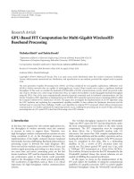
4. RESULTS
We implemented the proposed algorithm and tested its per-
formance on neurophysiological recordings obtained with
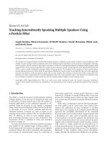
microelectrode arrays in the brain. In this specific applica-
tion, an array of microelectrodes is typically implanted in
the cortex to record neural activity from a small popula-
tion of neural cells as illustrated in the schematic of Figure 2.
The neural ac tivity of interest consists of short duration
signals (typically 1-2 ms in duration), often termed neural
“spikes” (due to their sharp transient nature), that occur ir-
regularly in the form of a spike train [9]. Each spike wave-
form is generated whenever the membrane potential exceeds
a certain threshold. The probability of spike generation de-
pends on the input the neuron receives from other neurons
in the population [36]. Generally speaking, neurons belong-

ing to the same population have near-identical waveforms
K. G. Oweiss and D. J. Anderson 7
Cell 1
Cell 2
Cell P
Biological signal
pathway
1
2
3
M
.
.
.
(a)
100 μm
Electrodes
(b)
Figure 2: (a) Schematic of a microprobe array of M electrodes monitoring neural activity from P adjacent neural cells in the central nervous
system. (b) A 64-channel Michigan electrode array with integrated elect ronics (amplification and bandpass filtering) on the back side of a
US 1 cent [35].
at the source. However, due to many factors, the waveform
from each neuron can be altered significantly due to the
anisotropic properties of the transmission medium (extra-
cellular space) [15]. The sensor array is generally designed
to record the activity of a small population of neural cells in
the vicinity of the array tip [35], thus the recordings are typi-
cally a mixture of multiple signal sources. The waveforms are
generally distinct at the sensor array and can be used to dis-
criminate between the orig inal sources. However, significant

correlation between the waveforms makes the separation task
extremely complex [37], especially without prior knowledge
of the exact waveform shape and the spatial distribution of
the sources.
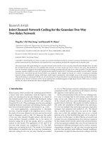
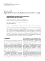
4.1. Signal and noise characteristics
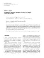
To illustrate some characteristics of this signal environment
with real data, typical neural signal char acteristics are illus-
trated in Figure 3 for long data record as well as sample wave-
forms extracted from them in Figure 4. The spectral and spa-
tial properties are also illustrated to demonstrate two impor-
tant facts: first, the signals are wide-band, in the sense that
the effective signal bandwidth is much larger than the recip-
rocal of the relative delay at which the signals are received
at the different sensors or different times. Second, if the ar-
ray is closely spaced, the signals tend to be largely coherent
across multiple adjacent electrodes. Moreover, the noise spa-
tial correlation extends over a much longer distance than the
signal spatial correlation, which rolls off rapidly as a function
of the distance between electrodes [10]. Sample spike wave-
forms are illustrated in Figure 4 to demonstrate their highly
correlated nature among multiple sources. The shape of each
waveform is a function of the source size, its distance from
the array and the unknown variable conductivity of the ex-
tracellular medium [15, 38].
A firm understanding of the signal milieu reveals the fol-
lowing categorization of the noise sources.
(a) Thermal, electrical noise due to amplifiers in the
headstage of the associated circuitry, and quantiza-
tion noise introduced by the data acquisition system.
This type can be regarded as a spatially and tempo-

rally white noise component belonging to the subspace
{Z}
⊥
.
(b) High levels of background activity caused by sources
far from the sensor array [39]. This noise type has spa-
tially correlated components ranging from localized
sources restricted to a subset of sensor array channels
(can be regarded as weak interference sources) to far
field sources engulfing the entire array. Both compo-
nents belong to the subspace
{Z}
//
.
4.2. Features obtained
We demonstrate two distinct signal sources along with their
sample waveforms recorded on a 4-channel electrode array
acquired experimentally in Figures 5 and 6,respectively.The
observation matrix in each case contains a single source, thus
P
= 1. We demonstrate in each figure the noisy spike wave-
form across channels along with its reconstructed waveform
from the best basis [26]. In each case, the source feature set
consists of the principal eigenmode
{λ
l
1
, u
l
1

} across the best
basis set J
1
.
8 EURASIP Journal on Advances in Signal Processing
0 102030405060708090
Time (ms)
100 μV
(a)
10
2
10
3
10
4
Frequency (Hz)
35
30
25
20
15
10
5
0
5
10
15
20
Power (dB)
Channel 1

Channel 2
Channel 3
Channel 4
(b)
020406080
Time (ms)
50 μV
(c)
10
2
10
3
Frequency (Hz)
50
45
40
35
30
25
20
15
10
5
Power (dB)
Channel 1
Channel 2
Channel 3
Channel 4
(d)
Figure 3: Characteristics of neural data measurements by a 4-elect rode array. Data in (a) panel is considered high SNR signals (SNR > 4dB),

while (c) panel is considered low SNR signals (SNR < 4 dB). The right panels illustrate the power spectral density of both data traces and
show that most of the spectral content of the noise matches that of the signal within the 10 Hz–10 kHz bandwidth but with reduced power
indicating that neural noise constitutes most of the noise process.
As mentioned previously, zero-valued λ
l
1
indicates sub-
band indices in which the l
2
-norm of the signal subspace,
in this case spanned by a single eigenvector u
l
1
,wasnot
adequately preserved. This means that the cost in (9)was
higher than the threshold needed to split the parent node.
Note that we used a linear indexing scheme for labeling tree
nodes for clarity. The averages displayed were calculated us-
ing a sample size of approximately 200 realizations of each
source.
Figure 7 illustrates the case when two sources were
present in the analysis interval. Careful examination of the
compound waveform in Figure 7(c) reveals that some mag-
nitude distortion occurs to source “B” wav eform (on channel
4) as a result of the overlap, while negligible distortion is no-
ticed for source “A” on channel 1. This is because the signal
subspace is clearly spanned by two distinct eigenvectors as
indicated by the selection of columns of the mixing matrix
as a
1

= [0.85 0.30 0.15 0.05] and a
2
= [0.05 0.10 0.20 0.80].
K. G. Oweiss and D. J. Anderson 9
300
250
200
150
100
50
0
50
100
150
200
μV
Source 1
Source 2
Source 3
Source 4
Source 5
Source 6
(a)
0 50 100 150
Distance (μm)
0
0.1
0.2
0.3
0.4

0.5
0.6
0.7
0.8
0.9
1
Normalized magnitude/correlation coefficient
Spike amplitude
Noise correlation (stimulus)
Noise correlation (no stimulus)
(b)
Figure 4: Temporal and spatial characteristics of the observed signal and noise processes. The left panel demonstrates six waveforms ex-
tracted from recordings of six distinct neurons. Waveforms have been cleaned by proper time alignment and averaging across multiple
realizations to display the templates shown.
246
Time (ms)
Observed
Reconstructed
(a)
(0)
(1)
(2)
(3)
(4)
(7)
(8)
(15)
(16)
(31)
(32)

(33)
(34)
(63) (64) (65) (66) (69) (70)
(b)
020406080
Node number
0
0.2
0.4
0.6
0.8
1
0.2
Normalized eigenvalue
(c)
1234
Channel
0
0.5
1
Signal subspace
(d)
Figure 5: (a) Single realization of a signal from source 1 along a 4-electrode array b efore and after best basis reconstruction (SNR = 4dB
and 10.8 dB, resp.). (b) Characteristic best basis wavelet packet tree (wavelet basis used was symlet of order 4). (c) Feature vector comprising
sample mean of λ
l
1
for 200 realizations (standard deviation is shown as error bars). (d) Sample mean of the principal eigenvector u
l
1

across
best tree nodes for the realization in (a).
10 EURASIP Journal on Advances in Signal Processing
246
Time (ms)
Observed
Reconstructed
(a)
0 20 40 60 80 100
Node number
0
0.2
0.4
0.6
0.8
1
Normalized eigenvalue
(b)
123 4
Channel
0
0.5
1
Signal subspace
(c)
(0)
(1)
(2)
(3) (4)
(7)

(8)
(9)
(10)
(15) (16) (17)
(18) (21)
(22)
(31)
(32)
(33)
(34) (35) (36) (37) (38) (43) (44)(45) (46)
63 64 65 66 6768 69 70 71 72 73 74 75 76 77 78 87 88 89 90 93 94
(d)
Figure 6: (a) Single source waveform along a 4-electrode array before and after best basis reconstruction (SNR = 5.7dBand10.8dB,resp.).
(b) Feature vector comprising sample mean of λ
l
1
for 200 realizations, standard deviation is shown as error bars. (c) Sample mean of the
principal eigenvector u
l
1
. (d) Characteristic best basis wavelet packet tree.
The first eigenmode {λ
l
1
, u
l
1
} is illustrated in Figure 7 in two
different ways. First, in Figure 7(d) the mode is displayed
across subbands similar to Figures 5 and 6.InFigure 7(e),

the eigenmode is displayed by reindexing the nodes based
on the decreasing order of magnitude of the eigenvalue λ
l
1
.
The purpose is to demonstrate how a threshold for λ
l
1
can
be selected such that the set J
1
can be determined. As in-
dicated by the MSE plot in Figures 7(d) and 7(e), the last
node, say j
∗
, for which the cost (9) is below a predetermined
threshold determines the minimum eigenvalue (dotted line
in Figure 7(e), top panel) that corresponds to a signal com-
ponent. It is clear that some nodes with indices j<j
∗
in
the ordered set (Figure 7(e), middle) do not correspond to a
minimum MSE. These nodes have eigenvalues λ
j
1
>λ
l
∗
1
but

their bases do not span the signal subspace. This is expected
since these bases span the subspace of the correlated com-
ponent of the two signals, which is stronger in these nodes
such that the dominant eigenvector points in the direction of
this component. These are eventually discarded from the set
J
1
.
Due to the sparsity introduced by the DWPT, the remain-
ing nodes in Figure 7(e) can b e clearly seen to span the sub-
space of source “B.” These nodes have eigenvalues that are
very close to zero as determined by the rank ordered λ
j
1
in
the top panel and correspond to maximum MSE. This obser-
vation can be further made by examining Figure 8 in which
the second eigenmode for the data matrix in Figure 7(c) is
illustrated.
The interpretation of these observations is fairly straight-
forward: the set J
1
is dominated by the 1st eigenmode, while
the remaining nodes with indices j/
∈ J
1
consist of two sub-
sets: one subset for which λ
j
1

is nonzero corresponds to ba-
sis spanning the “common” subspace of the two correlated
signals. The other subset corresponds to the other source,
K. G. Oweiss and D. J. Anderson 11
05
Time(ms)
+
(a)
05
Time (ms)
=
(b)
05
Time (ms)
(c)
0 20 40 60 80 100 120
Node number
Subband indexed 1st eigenmode of the
compound waveform
0
0.5
1
Normalized λ
0 20 40 60 80 100 120
0
0.5
1
1.5
Eigenvector
Channel 1

Channel 2
Channel 3
Channel 4
0 20 40 60 80 100 120
Node number
0
0.5
1
MSE
(d)
0 20 40 60 80 100 120
Reindexed Node number
Eigenvalue magnitude-indexed 1st eigenmode of the
compound waveform
0
0.5
1
Normalized λ
0 20 40 60 80 100 120
0
0.5
1
1.5
Eigenvector
Channel 1
Channel 2
Channel 3
Channel 4
0 20 40 60 80 100 120
Reindexed Node number

0
0.5
1
MSE
(e)
Figure 7: (a), (b) Template sources “A” and “B” across four channels with distinct mixing. Noise was filtered by averaging detected wave-
forms across 200 realizations. (c) Compound waveform obtained by summing the two signal matrices in (a) and (b). (d) 1st eigenvalue
(top) and eigenvector (middle) mode of the compound waveform across the DWPT tree. Most of the nonzero eigenvalues correspond to
eigenvectors that are similar to u
0
1
. In the bottom is the MSE between u
0
1
and u
j
1
, j = 0. It is clear that the error reaches a minimum in nodes
dominated by source “A.” (e) Same data in (d) based on arranging λ
j
1
in descending order of magnitude. This allows identifying a threshold
for λ
l
1
(as indicated by the arrow) that coincides with the last node j
∗
having a minimum distance u
j
∗

1
− u
0
1
.
which is regarded by the algorithm as “noise.” This inter-
pretation comes in perfect agreement with the vector space
interpretation described in Figure 1.
We have further examined the more complex case
where the signal subspaces are close. We selected a
1
=
[0.82 0.15 0.31 0.05] and a
2
= [0.82 0.15 0.11 0.05].
Figure 9 illustrates the features obtained. In this case, we
expected that the principal eigenmode
{λ
l
1
/u
l
1
} will alter-
nate between the two sets J
A
and J
B
(we used p = 1
to indicate source “A”andp

= 2 to indicate source
12 EURASIP Journal on Advances in Signal Processing
0 20 40 60 80 100 120
Node number
Subband indexed 2nd eigenmode of the
compound waveform
0
0.5
1
Normalized λ
0 20 40 60 80 100 120
0
0.5
1
1.5
Eigenvector
Channel 1
Channel 2
Channel 3
Channel 4
0 20 40 60 80 100 120
Node number
0
0.5
1
MSE
(a)
0 20 40 60 80 100 120
Reindexed Node number
Eigenvalue magnitude-indexed 2nd eigenmode of the

compound waveform
0
0.5
1
Normalized λ
0 20 40 60 80 100 120
0
0.5
1
1.5
Eigenvector
Channel 1
Channel 2
Channel 3
Channel 4
0 20 40 60 80 100 120
Reindexed Node number
0
0.5
1
MSE
(b)
Figure 8: (a) Second eigenmode of the compound waveform in Figure 7(c). The mode is arranged similar to Figure 7(d) based on linear
subband indexing. (b) Same features in (a) but reindexing the nodes based on descending order of magnitude of λ
j
2
. This allows identifying
a threshold for λ
l
2

(l ∈ J
2
, as indicated by the arrow) that coincides with the last node j
∗
in the sorted sequence having a minimum distance
u
j
∗
− u
0
2
.
“B” for clarity of notation) depending on which basis best
approximates the source with highest subband variance.
Specifically, let us consider the set of ordered nodes for
which λ
j
1
is nonzero. This includes roughly the ordered
nodes 0 to 22. In Figure 9(e) (middle panel), this set of
nodes can be divided in two subsets. The first subset (in-
cludes ordered nodes
{0, 1, 2, 3, 4, 5, 6, 9, 10, 13, 15,18, 22})
corresponds to an eigenvector spanning the same sub-
space as a
1
. The second subset (w hich includes ordered
nodes
{7, 8, 11, 12, 14, 16, 17, 19, 20, 21}) corresponds to the
eigenvector spanning the same subspace as a

2
. Mapping
these nodes back to their original linear indexing in the
binary tree yields the sets J
A
={0, 1, 3, 7, 15, 16} and
J
B
={4, 8, 10, 17, 18, 21}. Examining the tree structure
in Figure 9(f) illustrates that the nodes in each set follow
a parent-children relationship. Moreover, comparing these
nodes to the individual best basis t rees in Figures 5(b) and
6(d) for each individual source reveals that node indices be-
longing to J
B
are the ones that belong to source “B”anddo
not belong to those of source “A.”
The second eigenmode illustrated in Figure 10 corre-
sponds to the direction where the difference between the
signals is maximized. Specifically, let us examine each en-
try in the eigenvectors displayed in the middle panel of
Figure 10(b). Since unequal mixing was introduced only on
channel 3 (a
1
[3] = a
2
[3]), u
2
[3] is the largest entry. This is
expected since the second eigenvector should always point

in the direction of maximum difference between the signals.
In addition, u
2
[1] is nonzero because there is a difference in
the l
2
-norm of the original signals on channel 1 (Figures 9(a)
and 9(b)). Entry u
2
[2] (green) can be distinguished clearly in
nodes forming elements of the set J
A
, that is, those that are
dominated by source “A,” while this is not the case for the set
J
B
. This can be interpreted as channel 2 being the 3rd most
discriminating feature between the shapes of sources “A”and
“B,” after the unequal mixing on channel 3 and the distinct
norms on channel 1, respectively. Lastly, u
2
[4] is almost zero
since both signals are very weak on channel 4 and are equally
mixed.
4.3. Consistency and robustness
To assess the consistency and the robustness of the esti-
mated parameters, a simulation was carried out using the
spike templates illustra ted in Figure 11 in which five distinct
sources extracted from an array of four electrode channels
using proper spike alignment and averaging are displayed.

From this data, the “experimental” mixing matrix A could
be readily obtained. We used these templates to simulate a
data set with experimental noise extracted from the same
recordings. The spike train of each source was obtained from
a nonhomogenous Poisson process specifying the spike ar-
rival time stamps for each source [9]. These were stacked
in the rows of the signal matrix S, then premultiplied by
A. Noise variance was estimated from spike-free data from
the same experiment. Then, data below the noise variance
K. G. Oweiss and D. J. Anderson 13
05
Time (ms)
+
(a)
05
Time (ms)
=
(b)
05
Time (ms)
(c)
0 20 40 60 80 100 120
Node number
Subband indexed 1st eigenmode of the
compound waveform
0
0.5
1
Normalized λ
0 20 40 60 80 100 120

0
0.5
1
1.5
Eigenvector
Channel 1
Channel 2
Channel 3
Channel 4
0 20 40 60 80 100 120
Node number
0
0.1
0.2
MSE
(d)
0 20 40 60 80 100 120
Reindexed Node number
Eigenvalue magnitude-indexed 1st eigenmode of the
compound waveform
0
0.5
1
Normalized λ
0 20 40 60 80 100 120
0
0.5
1
1.5
Eigenvector

Channel 1
Channel 2
Channel 3
Channel 4
0 20 40 60 80 100 120
Reindexed Node number
0
0.1
0.2
MSE
(e)
(0)
(1)
(2)
(3) (4)
(7)
(8)
(9)
(10)
(15)
(16)
(17) (18) (21) (22)
(31)
(32)
(33)
(34)
(63) (64) (69) (70)
(f)
Figure 9: (a), (b) Template sources “A” and “B” with similar mixing, except for entry a
1

[3] = a
2
[3]. (c) Compound waveform obtained
by summing the two normalized signal matrices in (a) and (b). (d) 1st eigenmode of the compound waveform across the DWPT tree. The
nonzero eigenvalues correspond to eigenvectors that alternate between sources A and B subspaces. (e) 1st eigenmode of the compound
waveform displayed based on sorting λ
j
1
in descending order of magnitude. The set of ordered nodes up to node 22 can be seen to contain
two subsets, each subset has eigenvectors spanning the subspace of each of the two sources. The MSE in the bottom panel was calculated with
respect to a
1
. (f) Best basis binary tree using the first few eigenvalue ordered nodes. Nodes belonging to J
A
are circled, while those belonging
to J
B
are boxed.
14 EURASIP Journal on Advances in Signal Processing
0 20 40 60 80 100 120
Node number
Subband indexed 2nd eigenmode of the
compound waveform
0
0.5
1
Normalized λ
0 20 40 60 80 100 120
0
0.5

1
Eigenvector
Channel 1
Channel 2
Channel 3
Channel 4
0 20 40 60 80 100 120
Node number
0
0.1
0.2
MSE
(a)
0 20 40 60 80 100 120
Node number
Eigenvalue magnitude-indexed 2nd eigenmode of the
compound waveform
0
0.5
1
Normalized λ
0 20 40 60 80 100 120
0
0.5
1
Eigenvector
Channel 1
Channel 2
Channel 3
Channel 4

0 20 40 60 80 100 120
Node number
0
0.1
0.2
MSE
(b)
Figure 10: (a) 2nd eigenmode of the compound waveform in Figure 9(c). (b) Same data in (a) arranged in descending order of magnitude
of λ
j
2
.
was considered the colored noise component in the model
described in (1) and was superimposed on the product AS
yielding the observation matrix Y.
The conventional definition of SNR in neurophysiologi-
cal recordings is
SNR( dB)
= 20 log
10
Signal peak to peak amplitude
Noise RMS
. (16)
As mentioned previously, the nature of the neural spikes is
transient like, that is, comprises short duration events with
sharp edges of different magnitude and waveform shape de-
pending on the neural source relative location to the sensor
array. The numerator is calculated by estimating the average
peak-to-peak amplitude of spike waveforms detected on each
channel. The denominator is calculated from spike-free data

intervals as the noise root mean square. This helped assessing
the robustness of the algorithm for variable SNR.
We varied the sample size and the SNR. In Figure 12,esti-
mates of the signal subspaces are illustrated in (a). The vari-
anceoftheestimatesversusSNRforfixedsamplesizeisil-
lustrated in (b) for each source across channels. Note that
the variance was too small so it is plotted in dB for clarity.
It is clear that even in low SNR, the estimates exhibit very
small variance (∼
−50 dB) implying the robustness of the
estimates to degradation in SNR. The variances of the esti-
mated eigenvalues versus sample size are illustrated in Fig-
ures 12(c) and 12(d) for each source across channels. It is ob-
viously clear how a relatively small sample size of each source
leads to a robust estimation of the eigenvectors given the
observed small variance. The MSE between the true signal
subspace and the estimated one is illustrated in Figure 12(b)
for differentSNRsandvarioussamplesizesforeachsource.
At low SNR (up to 4 dB), the small sample size seems to af-
fect the estimates, but consistency is clear when the sample
size increases be yond 50 samples/source. On the other hand,
at high SNR (above 6 dB), the sample size does not seem to
affect the MSE at all and seems to attain the irreducible error
fairly quickly.
In Figure 13, we illustrate the variance of the eigenvalue
estimates across best basis nodes versus sample size. It can be
noticed that some nodes are sensitive to the small sample size;
while others do not seem to be affected and achieve conver-
gence relatively fast. The surprising result was the stabilit y of
some nodes at coarse scales (tree bottom) even though their

estimated eigenvalues are relatively the smallest entries in the
eigenvalue set λ
l
1
, l ∈ J
p
(refer to Figure 6(b) for an exam-
ple). This is very clear for source B for instance, which was
used in the example illustrated in Figure 6(a). On the other
hand, the SNR seems to affect the eigenvalue estimates to
some extent. This is clear from Figure 11(b), where the var i-
ance of the eigenvalue estimates is illustrated versus best tree
nodes for different SNR.
To summarize, the results show consistency of the esti-
mates as the sample size becomes large. The robustness of
the estimates is exceedingly high especially those of the sig-
nal subspace and does not seem to b e affected by the sample
size. Accordingly, one may argue that the separation process
can rely to a high degree of confidence on the signal subspace
K. G. Oweiss and D. J. Anderson 15
Channel 1Channel 2Channel 3Channel 4
Source A
(a)
Source B
(b)
Source C
(c)
Source D
(d)
Source E

(e)
Figure 11: Template waveforms for 5 neural sources extracted from experimental data used to assess the consistency of the estimated
parameters.
estimates in low SNR environments, since less variance of the
estimates is noticed. For example, from Figures 12(c) and
12(d), it is apparent that the variance converges rapidly to
the quantization noise level when the sample size is roughly
around 20 ∼ 25 samples/source for an SNR
= 2dB. More-
over, the observed variance can give some insight on the level
of classification error for a given spike sample size. On the
other hand, eigenvalues tend to be more stable when the SNR
is moderate to high regardless of the sample size.
4.4. Source detection
We have investigated the performance of the sphericity test
in (14) and compared it to classical source detection tech-
niques such as the AIC and MDL [40] in the context of
array processing [41, 42]. Figure 14 illustrates the perfor-
mance at multiple SNRs. We point out that one advantage
gained using the multiresolution sphericity test is the toler-
ance it allows for erroneous decisions. Specifically, if a noise
component predominates in a certain subband to the extent
of masking a weak source, then the sphericity test may under-
estimate P in that subband. In this case, the overall estimate
of P is minimally affected due to the fact that this source may
be better represented in another subband where the noise has
less masking effect thereby yielding a stronger mode that will
depend on how much correlation exists between that source
and the corresponding wavelet basis. The thresholds for the
sphericity tests are determined using the fact that the likeli-

hood function in (14) statistically approaches a Chi-square
distribution with (M
− p)
2
− 1 degrees of freedom [19].
4.5. Invariance to temporal nonstationarity
A well-known characteristic of neurophysiological recording
is the nonstationarity in the signals over short time periods.
This potentially occurs during bursting activity where it was
shown that the signal waveform can exhibit more than 50%
reductioninamplitude[43]. Typically, neural sources firing
successive spikes in a short period of time tend to introduce
observable attenuation in spike waveform shape due to the
16 EURASIP Journal on Advances in Signal Processing
ABCDE
Source
0
0.1
0.2
0.3
0.4
0.5
0.6
0.7
0.8
0.9
1
Signal subspace
Channel 1
Channel 2

Channel 3
Channel 4
(a)
AB C D E
Channel/source
500
450
400
350
300
250
200
150
100
50
0
Variance (dB)
2dB
4dB
6dB
8dB
10 dB
1234
(b)
Source A
0
0.5
1
10
4

Source B
0
2
4
10
3
Source C
0
2
4
10
3
Variance
Source D
0
2
4
10
4
Source E
0
2
4
10
3
0 50 100 150
Q (sample size/source)
Channel 1
Channel 2
Channel 3

Channel 4
(c)
Source A
2
4
10
2
Source B
5
10
10
2
Source C
45
120.8
10
3
MSE
Source D
2
6
10
2
Source E
2
6
10
2
20 40 60 80 100 120 140
Q (sample size/source)

2dB
4dB
6dB
8dB
10 dB
(d)
Figure 12: (a) Average estimates of u
l
p
for the neural sources in Figure 11 (SNR = 4 dB). (b) Variance of the estimates of u
l
p
versus SNR. (c)
Variance of the estimates of u
l
p
versus sample size (of spikes) for each source, for each channel (SNR = 2 dB). (d) MSE between the true u
l
p
and the estimated u
l
p
versus sample size versus SNR.
biophysical mechanism governing the concentration of the
ion channels within a neural cell and membrane potentials
[15, 44]. Long-term nonstationarity has been obser ved as
well due to cell migration, tissue relaxation, or electrode
encapsulation [38, 43]. Taken together, these temporal non-
stationarities can be regarded as a fading process that may
signficantly diminish the performance of any blind source

separation algorithm. Spatial nonstationarity has to be taken
into account as well especially when each neural source is
treated as a distributed source [34, 36]. This depends on the
neural cell type [44], or when migration of the recording ar-
ray relative to the neural population of interest occurs. How-
ever, temporal nonstationarity occurs at a faster rate com-
pared to spatial nonstationarity. The case of spatial nonsta-
tionarity can be fully accounted for by making the mixing
matrix time depedent. This case is outside the scope of this
K. G. Oweiss and D. J. Anderson 17
A
150
100
50
Q
0.01
0.04
0.08
B
150
100
50
Q
0
0.1
C
150
100
50
Q

0.01
0.03
0.05
D
150
100
50
Q
0
0.05
E
150
100
50
Q
0
0.05
0.1
Best tree nodes
(a)
A
10
6
2
SNR (dB)
0
0.05
B
10
6

2
SNR (dB)
0.02
0.04
0.06
10
6
2
SNR (dB)
0
0.05
D
10
6
2
SNR (dB)
0.01
0.03
0.05
E
10
6
2
SNR (dB)
0
0.05
Best tree nodes
(b)
Figure 13: (a) Variance of λ
l

1
, l ∈ J
p
(p ={A, B, C, D, E}), versus sample size Q (SNR = 4 dB) (b) Variance of λ
l
1
, l ∈ J
p
,versusSNR.(Nodes
with zero eigenvalues are suppressed for clarity.)
10
1
10
2
Number of snapshots (N)
0.1
0.2
0.3
0.4
0.5
0.6
0.7
0.8
0.9
Probability of detection error
AIC
MDL
MRST
6dB
9dB

Figure 14: Probability of error versus the number of snapshots for
the AIC, MDL, and multiresolution sphericity test in (14)[19].
paper. We will demonstrate that the algorithm is substantially
robust to temporal variations.
The signals in Figure 15 represent a single source with 50
realizations over time in a burst activity. The cleaned ver-
sion is illustrated for comparison. The multichannel signal
is illustrated in (c) for event number 26. In (d) through
(f), the features obtained a re demonstrated. The set J
1
was
invariant in all 50 realizations as well as the signal subspace
as illustrated in (c) and (f), respectively. On the other hand,
the eigenvalues λ
l
1
(k), 1 ≤ k ≤ 50, relative to the eigen-
value of the first realization λ
l
1
(1) clearly demonstrate that
the degradation in signal energy is efficiently captured by the
change in the eigenvalues. Most notably, the gradual decrease
in the eigenvalue in some nodes simultaneously occurs with
a gradual increase in the eigenvalue in others. It is also clear
that other nodes remain unchanged. These nodes can be in-
terpreted as ones that are insensitive to energy degradation
but rather capture other features in the waveform (e.g., zero
crossing) more efficiently than others.
5. CONCLUSION

The problem of blind source separation of unknown cor-
related sources from noisy observations has been analyzed.
We proposed a new solution to the problem that relies on
exploiting the spatial diversity of the communication chan-
nel. In the context of blind source separation, our goal was
to separate the correlated sources without having to estimate
the unknown channel. Specifically, we showed that eigende-
composition of orthogonal transformations of the unknown
signals is advantageous over classical time domain eigen-
decomposition when the orthogonality condition of signal
sources cannot be met. The orthogonal transformation was
carried out by means of the discrete wavelet transform and
its overcomplete representation, the discrete wavelet packet
transform, due of their excellent energy compaction ability.
This property introduces large sparseness in the t ransform
domain that constitutes a key element in reducing signal cor-
relation thereby allowing the signal subspace to be reliably
identified. We have further shown that the signal subspace
remains invariant under temporal nonstationary conditions
18 EURASIP Journal on Advances in Signal Processing
(0)
(1)
(2)
(3)
(4)
(7)
(8)
(15) (16)
(31)
(32)

(33)
(34)
(63) (64) (65) (66) (69) (70)
(a)
00.51 1.5
Time (ms)
200
150
100
50
0
50
100
150
200
μV
Noisy event number 1
00.511.5
Time (ms)
200
150
100
50
0
50
100
150
200
μV
50 noisy events

(b)
05
Time (ms)
100 μV
(c)
(0)
(1)
(2)
(3)
(4)
(7)
(8)
(15) (16)
(31)
(32)
(33)
(34)
(63) (64) (65) (66) (69) (70)
(d)
1 6 11 16 21 26 31 36 41 46
Spike event number
0
20
40
60
Best basis node number
Change in spectrotemporal
energy/first event (%)
Tre e to p
Tre e bottom

2
1
0
1
2
3
10
3
(e)
1 6 11 16 21 26 31 36 41 46
Spike event number
Spatial distribution
Channel 1
Channel 2
Channel 3
Channel 4
(f)
Figure 15: Tracking signal nonstationarity for an “attenuated-only” action potential of a bursting neuron. The largest amplitude spike is the
first event. The events on channel 1 are superimposed in (a) and (b) for comparison. (c) Observed signal across a 4-channel array for event
number 26. (d) Best basis tree set J
1
for each event. (e) The percentage change in eigenvalue λ
l
1
(k)relativetoλ
l
1
(1) magnitude across the
best basis set. T he circled nodes are the best subbands were the spike waveform is represented, and the combination of positive and negative
eigenvalues magnitudes changes in (e) is interpreted as a smooth migration of the spike projection from one node (where the change is

negative) to other nodes (where the change is positive). In the later, the spike projection becomes stronger despite the loss of energy in the
time domain waveform.
K. G. Oweiss and D. J. Anderson 19
of the signal, a property often observed in biological signals.
We also described one possible implementation of the algo-
rithm and showed its robustness to spatially and temporally
correlated noise processes. In the context of classification, the
approach utilizes a feature set that best describes the signal in
space, time, and scale using three components, namely, the
characteristic best basis binary tree set J
p
, the eigenvalue dis-
tribution λ
l
p
, l ∈ J
p
, and the principal eigenvector u
l
p
, l ∈ J
p
.
This case was not treated in detail and is reported elsewhere
[11].
Compared to MIMO systems, time and frequency diver-
sity were not exploited in this approach because of the nature
of the signal enviorment. It was assumed that the mixing is
instantaneous and the search for signal structures was con-
ducted across sensors. The particular case where noise is cor-

related with signals of interest is a major contribution of this
approach, often simplified in similar applications. It is also
obvious that the wavelet basis choice is of crucial importance
to the separation process and may not be trivial in some cases
since most wavelet bases share common properties like com-
pact support while differing in other properties like symme-
try and biorthogonality. The absence of knowledge about sig-
nal depedence complicates the problem to a large extent. For
this paper, we chose from a dictionary of bases reported in
the literature such as Haar, Daubechies, Symlet, Coiflet,and
so forth. Within a chosen basis, different versions exist de-
pending on the number of vanishing moments of the wavelet
function. On the other hand, when the signal structure is un-
available, symlets of small order seemed to yield the best per-
formance. We should note here that these results do not gen-
eralize for any sampling rate. The choice of another sampling
rate may render another basis to perform better than symlets.
One can argue that resampling the data to match a specific
wavelet basis may be helpful and may lead to better results.
When the signal is partially available in the form of signal
templates, they can be used to design admissible wavelet basis
to maximize a classification metric. Ideally, the wavelet basis
should be selected to provide maximum separability between
different sources. This topic is currently under investigation.
REFERENCES
[1] A. Hero, H. Messer, J. Goldberg, et al., “Highlights of statistical
signal and array processing,” IEEE Signal Processing Magazine,
vol. 15, no. 5, pp. 21–64, 1998.
[2] G. Bienvenu and L. Kopp, “Optimality of high resolution array
processing using the eigensystem approach,” IEEE Transactions

on Acoustics, Speech, and Signal Processing,vol.31,no.5,pp.
1235–1248, 1983.
[3] Y. Zhang, W. Mu, and M. G. Amin, “Subspace analysis of spa-
tial time-frequency distribution matrices,” IEEE Transactions
on Signal Processing, vol. 49, no. 4, pp. 747–759, 2001.
[4] A J. Van Der Veen, E. F. Deprettere, and A. L. Swindlehurst,
“Subspace-based signal analysis using singular value decom-
position,” Proceedings of the IEEE, vol. 81, no. 9, pp. 1277–
1308, 1993.
[5] P. Stoica, O. Besson, and A. B. Gershman, “Direction-of-
arrival estimation of an amplitude-distorted wavefront,” IEEE
Transactions on Signal Processing, vol. 49, no. 2, pp. 269–276,
2001.
[6] J. P. Le Cadre, “Parametric methods for spatial signal process-
ing in the presence of unknown colored noise fields,” IEEE
Transactions on Acoustics, Speech, and Signal Processing, vol. 37,
no. 7, pp. 965–983, 1989.
[7] P. Stoica, M. Viberg, and B. Ottersten, “Instrumental vari-
able approach to array processing in spatially correlated noise
fields,” IEEE Transactions on Signal Processing, vol. 42, no. 1,
pp. 121–133, 1994.
[8] H. Ye and R. D. DeGroat, “Maximum likelihood DOA esti-
mation and asymptotic Cramer-Rao bounds for additive un-
known colored noise,” IEEE Transactions on Sig nal Processing,
vol. 43, no. 4, pp. 938–949, 1995.
[9] F. Rieke, D. Warland, R. de Ruyter van Steveninck, and W.
Bialek, Spikes: Exploring the Neural Code, MIT Press, Cam-
bridge, Mass, USA, 3rd edition, 1997.
[10] K. G. Oweiss, “A systems approach for data compression
and latency reduction in cortically controlled brain machine

interfaces,” IEEE Transactions on Biomedical Engineering,
vol. 53, no. 7, pp. 1364–1377, 2006.
[11] K. G. Oweiss, “Integration of the temporal, spectral and spa-
tial information for classifying multi-unit extracellular neural
recordings,” IEEE Transactions on Biomedical Engineering,in
review
[12] K. G. Oweiss and D. J. Anderson, “A new technique for blind
source separation using subband subspace analysis in cor-
related multichannel signal environments,” in Proceedings of
IEEE International Conference on Acoustics, Speech and Signal
Processing (ICASSP ’01), vol. 5, pp. 2813–2816, Salt Lake City,
Utah, USA, May 2001.
[13] W. Hachem, F. Desbouvries, and P. Loubaton, “MIMO chan-
nel blind identification in the presence of spatially correlated
noise,” IEEE Transactions on Signal Processing, vol. 50, no. 3,
pp. 651–661, 2002.
[14] D. Kotoulas, P. Koukoulas, and N. Kalouptsidis, “Subspace
projection based blind channel order estimation of MIMO
systems,” IEEE Transactions on Signal Processing, vol. 54, no. 4,
pp. 1351–1363, 2006.
[15] C.Gold,D.A.Henze,C.Koch,andG.Buzs
´
aki, “On the ori-
gin of the extracellular action potential waveform: a model-
ing study,” Journal of Neurophysiology, vol. 95, no. 5, pp. 3113–
3128, 2006.
[16] D. Johnson and D. Dugeon, Array Signal Processing: Concepts
and Techniques, Prentice Hall, Englewood Cliffs, NJ, USA,
1st edition, 1993.
[17] A. K. Jagannatham and B. D. Rao, “Whitening-rotation-based

semi-blind MIMO channel estimation,” IEEE Transactions on
Signal Processing, vol. 54, no. 3, pp. 861–869, 2006.
[18] I. Daubechies, TenLecturesonWavelets, SIAM, Philadelphia,
Pa, USA, 1992.
[19] K. G. Oweiss, “Source detection in correlated multichannel
signal and noise fields,” in Proceedings of IEEE International
Conference on Acoustics, Speech and Signal Processing (ICASSP
’03), vol. 5, pp. 257–260, Hong Kong, April 2003.
[20] R. R. Coifman and M. V. Wickerhauser, “Entropy-based algo-
rithms for best basis selection,” IEEE Transactions on Informa-
tion Theory, vol. 38, no. 2, pt II, pp. 713–718, 1992.
[21] H. K. S. Mallat, D. Donoho, and A. S. Willsky, “Best basis al-
gorithm for signal enhancement,” in Proceedings of IEEE Inter-
national Conference on Acoustics, Speech and Signal Processing
(ICASSP ’95), vol. 3, pp. 1561–1564, Detroit, Mich, USA, May
1995.
[22] J C. Pesquet, H. Krim, and H. Carfantan, “Time-invariant or-
thonormal wavelet representations,” IEEE Transactions on Sig-
nal Processing, vol. 44, no. 8, pp. 1964–1970, 1996.
20 EURASIP Journal on Advances in Signal Processing
[23] P. L. Dragotti and M. Vetterli, “Wavelet footprints: theory, al-
gorithms, and applications,” IEEE Transactions on Signal Pro-
cessing, vol. 51, no. 5, pp. 1306–1323, 2003.
[24] M. S. Crouse, R. D. Nowak, and R. G. Baraniuk, “Wavelet-
based statistical signal processing using hidden Markov mod-
els,” IEEE Transactions on Signal Processing, vol. 46, pp. 886–
902, 1998.
[25] D. L. Donoho, “De-noising by soft-thresholding,” IEEE Trans-
actions on Information Theory, vol. 41, no. 3, pp. 613–627,
1995.

[26] K. G. Oweiss and D. J. Anderson, “A new approach to array de-
noising,” in Proceedings of the IEEE 34th Asilomar Conference
on Signals, Systems and Computers (ASSC ’00), vol. 2, pp.
1403–1407, Pacific Grove, Calif, USA, October-November
2000.
[27] D. B. Williams and D. H. Johnson, “Using the sphericity test
for source detection with narrow-band passive arrays,” IEEE
Transactions on Acoustics, Speech, and Signal Processing, vol. 38,
no. 11, pp. 2008–2014, 1990.
[28] T. Sugiyama, “On the distribution of the largest latent root of
the covariance matrix,” The Annals of Mathematical Statistics,
vol. 38, no. 4, pp. 1148–1151, 1967.
[29] T. Sugiyama, “On the distribution of the latent vectors for
principal component analysis,” The Annals of Mathematical
Statistics, vol. 36, no. 6, pp. 1875–1876, 1965.
[30] M. Vetterli and C. Herley, “Wavelets and filter banks: theory
and design,” IEEE Transactions on Signal Processing, vol. 40,
no. 9, pp. 2207–2232, 1992.
[31] Y. Suhail and K. G. Oweiss, “A reduced complexity integer
lifting wavelet-based module for real-time processing in im-
plantable neural interface devices,” in Proceedings of Annual
International Conference of the IEEE Enginee ring in Medicine
and Biology, vol. 2, pp. 4552–4555, San Francisco, Calif, USA,
September 2004.
[32] I. Daubechies and W. Sweldens, “Factoring wavelet transforms
into lifting steps,” Journal of Fourier Analysis and Applications,
vol. 4, no. 3, pp. 247–269, 1998.
[33] M W. Berry, “Large-scale sparse singular value computa-
tions,” International Journal of Super-Computer Applications,
vol. 6, no. 1, pp. 13–49, 1992.

[34] M. Nicolelis, Ed., Methods for Neural Ensemble Recordings,
CRC Press, Boca Raton, Fla, USA, 1998.
[35] K. Wise, D. Anderson, J. Hetke, D. Kipke, and K. Najafi, “Wire-
less implantable microsystems: high-density electronic inter-
faces to the nervous system,” Proceedings of the IEEE, vol. 92,
no. 1, pp. 76–97, 2004.
[36] E.R.Kandel,J.H.Schwartz,andT.M.Jessell,Eds.,Principles
of Neural Science, chapter 2, Appleton & Lange, Amsterdam,
The Netherlands, 3rd edition, 1991.
[37] M. S. Lewicki, “A review of methods for spike sorting: the de-
tection and classification of neural action potentials,” Network:
Computation in Neural Systems, vol. 9, no. 4, pp. 53–78, 1998.
[38] M. S. Fee, P. P. Mitra, and D. Kleinfeld, “Variability of extra-
cellular spike waveforms of cortical neurons,” Journal of Neu-
rophysiology, vol. 76, no. 6, pp. 3823–3833, 1996.
[39] M. S. Fee, P. P. Mitra, and D. Kleinfeld, “Automatic sorting of
multiple unit neuronal signals in the presence of anisotropic
and non-Gaussian variability,” Journal of Neuroscience Meth-
ods, vol. 69, no. 2, pp. 175–188, 1996.
[40] J. Rissanen, “Modeling by shortest data description,” Automat-
ica, vol. 14, no. 5, pp. 465–471, 1978.
[41] W.Chen,K.M.Wong,andJ.P.Reilly,“Detectionofthenum-
ber of signals: a predicted eigen-threshold approach,” IEEE
Transactions on Signal Processing, vol. 39, no. 5, pp. 1088–1098,
1991.
[42] Y. Wu and K W. Tam, “On determination of the number of
signals in spatially correlated noise,” IEEE Transactions on Sig-
nal Processing, vol. 46, no. 11, pp. 3023–3029, 1998.
[43] G. Buzs
´

aki, “Large-scale recording of neuronal ensembles,”
Nature Neuroscience, vol. 7, no. 5, pp. 446–451, 2004.
[44] K. D. Harris, D. A. Henze, J. Csicsvari, H. Hirase, and
G. Buzs
´
aki, “Accuracy of tetrode spike separation as deter-
mined by simultaneous intracellular and extracellular mea-
surements,” Journal of Neurophysiology, vol. 84, no. 1, pp. 401–
414, 2000.
Karim G. Oweiss obtained his B.S. (1993)
and M.S. (1996) degrees in electrical en-
gineering from the University of Alexan-
dria, Egypt, and the Ph.D. degree in electri-
cal engineering and computer science from
the University of Michigan, Ann Arbor, in
2002. His Ph.D. dissertation exploited mul-
tiresolution analysis of multichannel neu-
ral recordings. He completed a postdoctoral
training with the Biomedical Engineering
Department at the University of Michigan, Ann Arbor in the sum-
mer of 2002. In August 2002, he joined the Department of Electrical
and Computer Engineering at Michigan State University, where he
is currently an Assistant Professor and Director of the Neural Sys-
tems Engineering Laboratory. His research interests include statis-
tical signal processing, information theory, data mining, multires-
olution analysis, fast DSP algorithms with primary applications to
neural signal processing, computational neuroscience, and brain
machine interface technology. He is a Member of the IEEE, the
Society for Neuroscience and the International Society for Opti-
cal Engineering. He is also a Member of the technical committee of

the IEEE Signal Processing Society, the IEEE Circuits and Systems
Society, and the IEEE Engineering in Medicine and Biology Society.
David J. Anderson received the B.S.E.E. de-
gree from Rensselaer Polytechnic Institute,
Troy,NY,andtheM.S.andPh.D.degrees
from the University of Wisconsin, Madison.
After completing a postdoctoral traineeship
with the Laboratory of Neurophysiology,
University of Wisconsin Medical School, he
joined the University of Michigan, Ann Ar-
bor, where he is now a Professor of electrical
engineering and computer science, biomed-
ical engineering, and otolar y ngology. His research is in the areas
of auditory physiology, neural recording device design, and signal
processing of neural recordings. He is the founding Director of the
University of Michigan Center for Neural Communication Tech-
nology, which conducts research on the development and use of
silicon neural probe technology and distributes devices to neuro-
scientists worldwide. He is a Fellow of the American Institute for
Medical and Biological Engineering, a Member of the Neuroscience
Society, the Association for Research in Otolar yngology, and the
Barany Society.