Hindawi Publishing Corporation
EURASIP Journal on Advances in Signal Processing
Volume 2007, Article ID 24717, 12 pages
doi:10.1155/2007/24717

Research Article
MAP-Based Underdetermined Blind Source Separation
of Convolutive Mixtures by Hierarchical Clustering
and 1-Norm Minimization
Stefan Winter,1, 2 Walter Kellermann,2 Hiroshi Sawada,1 and Shoji Makino1
1 NTT

Communication Science Laboratories, Nippon Telegraph and Telephone Corporation, 2-4 Hikaridai, Seika-Cho,
Soraku-Gun, Kyoto 619-0237, Japan
2 Multimedia Communications and Signal Processing, University of Erlangen-Nuremberg, CauerstraBe 7,
91058 Erlangen, Germany
Received 30 September 2005; Revised 24 January 2006; Accepted 11 June 2006
Recommended by Frank Ehlers
We address the problem of underdetermined BSS. While most previous approaches are designed for instantaneous mixtures, we
propose a time-frequency-domain algorithm for convolutive mixtures. We adopt a two-step method based on a general maximum
a posteriori (MAP) approach. In the first step, we estimate the mixing matrix based on hierarchical clustering, assuming that the
source signals are sufficiently sparse. The algorithm works directly on the complex-valued data in the time-frequency domain
and shows better convergence than algorithms based on self-organizing maps. The assumption of Laplacian priors for the source
signals in the second step leads to an algorithm for estimating the source signals. It involves the 1 -norm minimization of complex
numbers because of the use of the time-frequency-domain approach. We compare a combinatorial approach initially designed for
real numbers with a second-order cone programming (SOCP) approach designed for complex numbers. We found that although
the former approach is not theoretically justified for complex numbers, its results are comparable to, or even better than, the SOCP
solution. The advantage is a lower computational cost for problems with low input/output dimensions.
Copyright © 2007 Stefan Winter et al. This is an open access article distributed under the Creative Commons Attribution License,
which permits unrestricted use, distribution, and reproduction in any medium, provided the original work is properly cited.

1.

INTRODUCTION

The high-quality separation of speech sources is an important prerequisite for further processing such as speech recognition in environments with several active speakers. Often,
the underlying mixing process is unknown, thus requiring
blind source separation (BSS). In general, we can distinguish
two cases depending on the number of sources N and the
number of sensors M:
(i) N > M: underdetermined BSS,
(ii) N ≤ M: (over-) determined BSS.
Since overdetermined BSS (N < M) can be reduced to determined BSS (N = M) [1], we refer to both as determined
BSS. Most approaches deal with determined BSS [2, 3], but in
reality BSS is often underdetermined. While the area of underdetermined BSS is attracting increasing attention [4–12],
it remains a challenging task.
Most existing approaches for underdetermined BSS were
proposed for instantaneous mixtures. In this paper, we use

[13, 14] as our basis for proposing an algorithm for underdetermined BSS that deals with convolutive mixtures in the
time-frequency domain. We start from a general Bayesian approach, which leads to a two-stage framework. In the first
stage, we have to estimate the mixing matrix. In the second,
stage the actual source signals are estimated.
Several of the previously proposed algorithms for the
first stage are based on histograms and developed for only
two sensors [7, 9, 11]. Some could, in principle, be enhanced for higher dimensions M. But since histograms are
based on densities, the so-called curse of dimensionality
[15] sets practical limits to the number of usable sensors.
This problem becomes even worse with complex numbers,
which double the histogram dimensions due to their real
and imaginary parts or amplitude and phase, respectively.

Complex numbers are necessary if BSS is performed in the
time-frequency domain. Some methods approach complex
numbers by applying real-valued algorithms to the real and
imaginary parts or amplitude and phase [6, 12], which is not
always applicable. Some approaches extract features such as


2

EURASIP Journal on Advances in Signal Processing

the direction of arrival (DOA), or work on the amplitude relation between two sensor outputs [4, 5, 7, 16]. In both cases,
only two sensors can contribute, no matter how many sensors are available.
Other algorithms such as GeoICA [8] or AICA [10] resemble self-organizing maps (SOMs) and could more easily
be applied to convolutive mixtures. However, their convergence depends heavily on initial values [15]. Usually, countermeasures are computationally expensive.
Here we propose the use of hierarchical clustering to estimate the mixing matrix. This method can work directly on
complex-valued samples. While it does not limit the usable
numbers of sensors, it prevents the convergence problems
that can occur with SOM-based algorithms.
In the second stage, we separate the mixtures using the
estimated mixing matrix from the first stage. We assume statistical independence and Laplacian probability density functions (PDFs) for the sources [17]. This leads to constrained
1 -norm minimization. Since we are considering convolutive
mixtures, we work in the time-frequency domain. This reduces the convolutive mixtures to instantaneous mixtures,
which are easier to handle. As a result, we have to deal with
complex numbers.
Therefore we investigate the difference between real- and
complex-valued 1 -norm minimizations and its implication
for the underdetermined BSS of convolutive mixtures.
In Section 2, we first explain the general framework before providing details about the hierarchical clustering in
Section 3 and the source separation based on 1 -norm minimization in Section 4. In Sections 4.2 and 4.3, we present

a detailed description of real- and complex-valued 1 -norm
minimizations before considering their differences. The consequences of these differences for practical applications are
described in Section 5 together with experimental results.
They demonstrate the performance for convolutively mixed
speech data in a real room with reverberation time TR = 120
milliseconds.
2.

GENERAL FRAMEWORK

We consider a convolutive mixing model with N speech sources si (t) (i = 1, . . . , N) and M (M < N) sensors that yield
linearly mixed signals x j (t) ( j = 1, . . . , M). The mixing can
be described by
N

∞

x j (t) =

h ji (l)si (t − l),

(1)

i=1 l=0

where h ji (t) denotes the impulse response from source i to
sensor j.
Instead of solving the problem in the time domain, we
choose a narrowband approach in the time-frequency domain by applying a short-time Fourier transform (STFT).
While a wideband approach would be desirable, extension of

the proposed method is not as straightforward as described
for example in [18]. This is because this problem has a different structure from traditional adaptive filtering problems.
Following [13], we can approximate the mixing process in

the time-frequency domain as
X( f , τ) = H( f )S( f , τ),

(2)

where X ∈ KM , H ∈ KM ×N , S = [S1 , . . . , SN ]T ∈ KN , K = C,
and τ denotes the time frame.
This reduces the problem from convolutive to instantaneous mixtures in each frequency bin f . For simplicity, we
will omit the frequency and time-frame dependence. Switching to the time-frequency domain has the additional advantage of making it easier to exploit the time-frequency sparseness of speech sources [6]. Sparseness of a signal means that
only a few instances have a value significantly different from
zero. During speech activity, the amplitude of a speech signal in the time domain is usually significantly different from
zero, and therefore not sparse. The higher sparseness in the
time-frequency domain can be explained by the harmonic
structure of speech signals. During voiced speech, the energy of a speech signal is concentrated around multiples of
the speaker’s fundamental frequency. Ideally, the frequency
bands in between do not carry any energy. This means that in
the time-frequency domain, only a few frequency bins have
high values at each time instance τ, while most frequency
bins have a value close to zero. This is by definition a sparse
signal. In addition, the fundamental frequency depends on
the time instance τ, which means that the signal is also sparse
with respect to τ. Together with the frequency sparseness and
the speaker dependency, this leads to less overlap in the timefrequency domain than in the time domain. Using a sparse
signal representation is very important as regards ensuring
good separation performance since the separation is built on
the assumption of sparse source signals.

The disadvantage of narrowband BSS in the timefrequency domain is the internal permutation problem,
which results in incorrect frequency bin alignment. In our
framework, we use a clustering-based method to reduce the
permutation problem [3, 19]. We also apply the minimumdistortion principle [2] to solve the scaling problem.
In determined BSS, the mixing matrix H is square and
(assuming full rank) invertible. Therefore, the BSS problem
can be solved by either inverting an estimate of the mixing
matrix or directly estimating its inverse and solving (2) for S.
However, this approach does not work in underdetermined BSS where the mixing matrix is not invertible. Instead,
we follow a general Bayesian approach, which leads to an optimal solution in a statistical sense. In general, we search for
an estimation of the source signals S and mixing matrix H
that maximize the a posteriori P(S, H|X). If we make the usually reasonable assumption that the source signals and mixing matrix are statistically independent, this problem can be
written as

max P(S, H | X) = max
S,H

S,H

P X | S, H P(S, H)
P(X)

∼ max P(X | S, H)P(S)P(H).
S,H

(3)
(4)


Stefan Winter et al.


3
s(t)

Inverse
STFT

S( f , τ)

X( f , τ)
STFT

x(t)

BSR

H
Permutation

BMMR

Figure 1: Overall unmixing system.

If we assume additive white Gaussian noise with variance ν2
at the sensors, then the likelihood P(X|S, H) also has a Gaussian distribution according to
P(X | S, H) = N X | HS, ν2 I .

(5)

We will limit ourselves to the noiseless case (ν2 → 0), which

leads to a Dirac impulse for the likelihood
P(X | S, H) = lim N X | HS, ν2 I = δ(X − HS).
2
ν →0

(6)

It requires the maximum of the a posteriori to fulfill HS = X,
which turns (3) into the constrained problem
max P(S)P(H)
S,H

s.t. HS = X.

(7)

If we further assume that we know the mixing matrix H (or
can provide an estimate for it as shown in Section 3), then
P(H) is also a Dirac impulse. So we only have to estimate the
source signals S, and (7) results in
max P(S)
S

s.t. HS = X.

(8)

Therefore we follow a two-stage approach as utilized in [6, 8]
consisting of blind mixing model recovery (BMMR) and
blind source recovery (BSR). To estimate the mixing matrix

A in the BMMR step, we propose the use of hierarchical clustering as described in detail in Section 3. To eventually separate the signals in the BSR step, we specify a source model
P(S) and provide a solution for (8) in Section 4. Finally, the
inverse STFT is applied to obtain time-domain signals. The
overall system is depicted in Figure 1.

This means that each time-frequency instance originates only
from a single source and represents a scaled version of the
corresponding mixing vector hq ( f ). q depends on the frequency f and time τ.
If we assume stationary source positions, the mixing vector hq ( f ) is constant for all τ. Since hq ( f ) is related to the
position of the qth source, it is also different for each source.
This means ideally that the time-frequency samples X( f , τ),
that originate from the qth source, cluster at each frequency
f around the corresponding mixing vectors hq ( f ).
However, depending on the mixing system and the actual
time-frequency sparseness of the source signals, the mixed
signals will also have components of other mixing vectors
stemming from other sources. Therefore the mixtures will be
spread around the mixing vectors but still form clusters for
each source.
3.1.

Hierarchical clustering

To avoid the problems discussed in Section 1, such as the
curse of dimensionality or poor convergence, we propose
the use of a hierarchical clustering algorithm for finding the
clusters around the mixing vectors. We follow an agglomerative (bottom-up) strategy. [15]. This means that the starting
point is the single samples, considering them as clusters that
contain only one object. Clusters are then combined, so that
the number of clusters decreases while the average number

of objects per cluster increases. In the following, we assume
phase and amplitude normalized samples
X ←−

3.

BLIND MIXING MODEL RECOVERY

Several algorithms have already been proposed for BMMR.
They usually have the common feature that they assume
sparseness of the original signals. Without being mentioned,
it is usually assumed that the sources are located at different
spatial positions (space sparseness). In addition, they commonly assume a certain degree of time-frequency sparseness,
which ideally means that the time-dependent spectra of the
sources do not overlap even after being mixed. Rewriting (2),
we can express ideal time-frequency sparseness by
N

X( f , τ) =

hi ( f )Si ( f , τ)

(9)

i=1

= hq ( f )Sq ( f , τ),

q ∈ {1, . . . , N }.


X
|X |2

e−ϕX1 ,

(10)

where ϕX1 denotes the phase of the first vector component of
X and |·| p denotes the p -norm defined by
1/ p
p

|Z| p =

Zi

.

(11)

i

The combination of clusters into new clusters is an iterative
process based on the distance between the current clusters.
Starting from the normalized samples, the distance between
each pair of clusters is calculated, resulting in a distance matrix. At each level of the iteration, the two clusters with the
least distance are combined to form a new binary cluster
(Figure 2). This process is called linking and is repeated until the number of clusters has decreased to a predetermined
value c, N ≤ c ≤ P (P is the total number of samples).



4

EURASIP Journal on Advances in Signal Processing

0.3

10
9
c 8
7
6
5
4
3
2
1

Level

Imaginary (X2 )

0.2

1

2

3


4

5

6
7
Object

8

9

10

11

0.1
0

 0.1
 0.2
 0.3
0

0.1

0.2

0.3


Figure 2: Linking the closest clusters.

0.4
0.5
Real (X1 )

0.6

0.7

0.8

Estimated hi
Original hi
d(C1 , C2 )

Figure 4: Estimation of mixing vectors, f = 1164 Hz.

C2

C1
d(Xτ1 , Xτ2 )

Figure 3: Illustration of distances.

To measure the distance between clusters, we have to
distinguish between two different problems. First we need
a distance measure d(Xτ1 , Xτ2 ) that is applicable to Mdimensional complex vector spaces. While there are several
possibilities, we currently use the Euclidean distance based
on the normalized samples, which is defined by

d Xτ1 , Xτ2 =

Xτ1 − Xτ2 , Xτ1 − Xτ2

∗

,

(12)

where ·, · stands for the inner product and ∗ stands for
complex conjugation.
When a new cluster is formed, we need to enhance
this distance measure to relate the new cluster to the other
clusters. The method we employ here is called the nearestneighbor technique. Let C1 and C2 denote two clusters as
illustrated in Figure 3. Then the distance d(C1 , C2 ) between
these clusters is defined as the minimum distance between its
samples by
d C 1 , C2 =

min

Xτ1 ∈C1 , Xτ2 ∈C2

d Xτ1 , Xτ2 .

(13)

As mentioned earlier, most of the samples will cluster around
the mixing vectors hi , depending on the degree of sparseness of the original signals. Special attention must be paid to

the remaining samples (outliers), which are randomly scattered in the space between the mixing vectors due to nonideal
sparseness (and noise if applicable). Usually they are far away
from other samples and will be combined with other clusters
only at higher levels of the clustering process (i.e., when only
few clusters are left). This led us to the idea of setting the final
number of clusters at a high value:
c

N.

(14)

By doing so, we avoid linking these outliers with the clusters
around the mixing vectors hi and therefore avoid distortions.
This results in greater robustness. More important, however,
is the fact that we avoid combining desired clusters. Since the
outliers are often far away from other clusters, desired clusters might be closer to each other than to outliers. Experiments showed that the exact value of c does not matter as
long as it is above 60 for N ∈ {3, 4, 5}.
This approach requires distance calculations, but with a
well-designed implementation as used here, the computational complexity can become as low as O(n2 ) [20], where
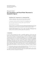
n denotes the number of samples per frequency bin. An example of the resulting clusters is shown in Figure 4. Here, as
with the experiments in Section 5, we chose c = 100. An
example where desired clusters were unintentionally combined because too small a value c was chosen is shown in
Figure 5. Further experimental details are given in Section 5.
3.2.

Estimation of mixing matrix

Assuming that the clusters around the mixing vectors hi have
the highest densities, and therefore the highest numbers of

samples, we finally chose the N clusters with the largest numbers of samples. Thereby, the number of sources N must be
known. To obtain the mixing vectors, we average over all the
samples of each cluster,
hi =

1
Ci

X,

1 ≤ i ≤ N,

(15)

X∈Ci

where |Ci | denotes the cardinality of cluster Ci . Thereby, we
assume that the influence of other sources has zero mean.
3.3.

Advantages of hierarchical clustering

Among the most important advantages of the above hierarchical clustering algorithm is the fact that it works directly
on the sample data in any vector space with arbitrary dimensions. The only requirement is the definition of a distance


Stefan Winter et al.

5
and amplitudes with uniform and one-sided Laplacian distributions, respectively, the cost function results in


0.3

Imaginary (X2 )

0.2
S

i = 1, . . . , N,

s.t. HS = X,

(16)

i

0

for each time instance τ. |Si | denotes the amplitude of Si .

 0.1
 0.2

4.2.

 0.3
0

0.1


0.2

0.3

0.4
0.5
Real (X1 )

0.6

0.7

0.8

Estimated hi
Original hi

Figure 5: Example of unintentionally combining desired clusters,
f = 1164 Hz.

measure for the considered vector space. Therefore, it can
easily be applied to the complex-valued data that occurs in
time-frequency domain convolutive BSS.
No initial values are required for the mixing vectors hi .
This means, in particular, that if the assumption of clusters
with high densities around the mixing vectors is true, then
the algorithm converges to those clusters.
Besides choosing a distance measure, there is only the
single parameter c that determines the number of clusters.
Experiments have shown that the choice of this parameter

is quite insensitive as long as it is above a certain limit that
would combine desired clusters. Its choice is, in general, related to the sparseness of the sources. The sparser the signals
are, the smaller the value of c can be, because the number of
outliers that must be avoided will be smaller.
While the considered signals must have some degree of
sparseness, they do not have to be statistically independent
at this point to obtain clusters.
4.

|Si |,

min

0.1

BLIND SOURCE RECOVERY

Unmixed signals cannot be directly obtained, because the
mixing matrix cannot be inverted in underdetermined BSS.
Several approaches have been proposed to solve blind source
recovery [17]. Of these approaches, we chose the shortestpath algorithm, which is based on maximum a posteriori
(MAP) estimation, assuming statistical independence and
Laplacian PDFs for the sources.
4.1. MAP-based cost function
Using a maximum a posteriori (MAP) approach, we have
shown in Section 2, that once we know the mixing matrix
H, we have to solve the constrained problem (8) in order to
obtain a statistically optimal estimate for the source signals
S. If we assume mutually independent source signals whose
spectral components have statistically independent phases


1 -norm minimization of real-valued problems

If we had to consider only real-valued problems (K = R), we
could employ linear programming (LP) [21], which solves
problems of the form
min cT S,

s.t. HS = X,

Si ≥ 0,

i = 1, . . . , N,

(17)

where c, S ∈ RN , H ∈ RM ×N , and X ∈ RM . For K = R,
(16) can be transformed into (17) by separating positive and
negative values by
S ←−

S+
,
S−
(18)

1
c ←−
,
1


H
H ←−
,
−H

X ←− X.

Here 1 stands for a unity matrix with appropriate dimensions. S+ and S− are derived from S by setting all negative
values or positive values, respectively, at zero.
Although powerful algorithms for linear programming
exist, they are still time consuming. Depending on the dimensions of the problem, we can obtain a faster combinatorial algorithm if we use a certain property of the solution. It
can be shown [8, 22] that the N-dimensional vector S that
solves (16) contains at least N − M zeros if the columns of H
are normalized. The normalization can be assumed for BSS
due to the scaling ambiguity.
The lower limit for the number of zeros can be considered a constraint imposed by the MAP estimation and can
easily be fulfilled by setting N − M elements of the solution
at zero. Then we only have to determine the remaining M elements. Assuming that we know where to place the zeros, the
remaining elements are found by multiplying the inverse of
the quadratic matrix built by the remaining mixing vectors
hi with the constraining vector X:
hi 1 , . . . , hi M

−1

X,

i1 , . . . , iM ∈ {1, . . . , N }.


(19)

The correct placement of the zeros can be determined by
combinatorially testing all possibilities and accepting the one
with the smallest 1 -norm. As a simple example, let us consider
H=

1 0.6 −0.6
,
0 0.8 0.8

X=

1
.
0.5

(20)

According to the dimensions of the problem, at least one element of the solution S must be zero. The 1 -norm of the


6

EURASIP Journal on Advances in Signal Processing

possible solutions is

By defining
⎡


⎡

−1

1 0.6

⎢
⎢
⎣ 0 0.8

⎤

1 ⎥
0.5 ⎥
⎦

0
⎡

1 −0.6
0 0.8

⎣0
⎡

0

⎢
⎢ 0.6 −0.6

⎣

0.8 0.8

= 1.25,

(21)

1
−1

⎤

1 ⎦
0.5

= 2,

(22)

1

−1

⎥
c1 ⎥
⎦

0.5


= 1.6.

=

0
0

|S|1 ≤ t.

(24)

h1
h1

min cT S,

i=1

Si

|S|1 =

≤ 1T t = 1T t1 , . . . , tN

T

= t,

(25)


2

s.t. X = HS,

Si
Si

≤ ti ,
2

∀i. (26)

··· 0
··· 0

−

hN
hN

hN
∈ R2M ×3N ,
hN
(27)

Si
Si

≤ ti


∀i. (28)

2

The second constraint in (28) can be interpreted as a secondorder cone for each i.
Equation (28) describes an SOCP problem [24], which
can be solved numerically for example with SeDuMi [16].
Analysis of real- and complex-valued
1 -norm minimizations

In contrast to the real-valued 1 -norm minimization problem where a minimum number of zeros can be guaranteed
theoretically in the optimal solution, the number of zeros
cannot be predicted with complex-valued problems as the
following simple example shows. Let
⎡

⎤

4
17 ⎥
⎢
⎥
⎥,
H=⎢
⎣
0.8 + j0.6 ⎦
√
0 0.8
17
⎢1 0.6


Then the
by

1 -norm

√

Ssocp

X=

1
.
0.5

(29)

of the solution obtained by SOCP is given
⎤

⎡

0.227 + 0.040i
⎥
⎢
⎢0.511 − 0.091i⎥
⎦
1 = ⎣
0.481 + 0.015i


= 1.23.

(30)

1

It does not contain any zeros as we would expect with
real numbers, yet it solves (16). In comparison, the 1 -norm
of the optimal combinatorial solution is given by
⎡

Scomb

t

h1
h1

S

where (·) and (·) denote the real and imaginary parts,
respectively. Thus we can rewrite (16) as

min 1T t,

−

s.t. X = HS,


By decomposing t = N 1 ti , ti ∈ R, the second constraint
i=
|S|1 ≤ t can be expressed by
Si

(X)
∈ R2M ,
(X)

we can write

4.4.

If complex numbers are involved, then (18) can no longer be
applied because such numbers possess a continuous phase in
contrast to a discrete phase of real numbers. Thus we cannot
use algorithms that solve linear programming problems for
complex-valued problems. However, 1 -norm minimization
problems (16) with complex numbers (K = C) can be transformed to second-order cone programming (SOCP) problems in the following way.
Equation (16) is equivalent to

N

0

H

1

s.t. X = HS,


c1

⎢ ⎥
⎢0⎥
⎢ ⎥
⎢0⎥
⎢ ⎥
⎢ ⎥
⎢.⎥
c = ⎢ . ⎥ ∈ R3N ,
⎢.⎥
⎢ ⎥
⎢1⎥
⎢ ⎥
⎢ ⎥
⎣0⎦

⎥
⎥
⎥
⎥
⎥
⎥
⎥
⎥ ∈ R3N ,
⎥
⎥
⎥
⎥

⎥
⎦

X=

(23)

1 -norm minimization of complex-valued
problems

min t ∈ R,

⎡ ⎤

⎤

⎤

The notation of (22) reflects the above description of setting
one element at zero and inverting the remaining quadratic
matrix. The chosen solution would be the one corresponding
to (21).
This combinatorial method is based on the shortestpath algorithm [8] and the 0 -norm that basically counts
the number of nonzero elements. The combinatorial method
stands in contrast to the approach in [23] where conditions
are given for which the 0 -norm can be calculated by an p norm with 0 < p ≤ 1.
4.3.

ct1
S1

S1
.
.
.
tN
SN
SN

⎢
⎢
⎢
⎢
⎢
⎢
⎢
S=⎢
⎢
⎢
⎢
⎢
⎢
⎣

1

0

⎢⎡
⎤−1
⎢

4
⎢ 0.6
√
= ⎢⎢
1
17 ⎥
⎢⎢
⎥
⎢⎢
⎥
⎣⎣
0.5
0.8 + j0.6 ⎦
√
0.8

17

⎤
⎥
⎥
⎥
⎥
⎥
⎥
⎦

= 1.24.
1


(31)


Stefan Winter et al.

7

X = HScomb = HSsocp .

1.27
1.265
1.26
1 -norm

This observation reveals a very important difference from
real-valued problems and prevents the theoretical justification of a procedure similar to the combinatorial approach in
Section 4.2. To better explain this difference between real and
complex numbers, we take a look at a general solution based
on a combinatorial solution and the nullspace N (H) of H.
Even though the combinatorial solution Scomb does not
necessarily minimize the 1 -norm, it fulfills together with the
SOCP solution Ssocp that

1.24
1.235
0

(34)

with

S ∈ N (H) ⇐⇒ S = 1 − H− H z, z ∈ CN ,

(35)

where H− is an arbitrary generalized inverse of H. For N = 3
and M = 2, we can express the combinatorial solution and
the nullspace without loss of generality by

⎡

h h
N (H) = α ⎣ 1 2
1

−1

⎤

X⎦

,
(36)

⎤

h3 ⎦

,

1


=

f11 (H, X) + α f12 (H, X)
+ f21 (H, X) + α f22 (H, X)

Sensor distance
Source signal length
Reverberation time TR
Sampling frequency fs
Window type
Filter length
Shifting interval
Number of clusters c

0.25

(37)

+ f31 (H, X) + α f32 (H, X) .
Here fi j is a summand that only depends on H and X, which
are constant for any given problem. If only real values are
involved, then (37) describes a piecewise linear function depending on α whose slope can only change a limited number
of times in a discrete manner.
However, once complex numbers are involved, their
imaginary part results in an inherent 2 -norm, which leads
to smooth slopes as they appear with second-order or higher
polynomials. This behavior becomes obvious in (28). There
the 1 -norm is changed from the sum of the absolute values of real numbers to the sum of the 2 -norms of the
real and imaginary parts. The introduction of the 2 -norm

explains the different behavior of complex-valued 1 -norm

40 mm
7 seconds
120 ms
8 kHz
von Hann
1024 points
256 points
100

minimization compared with its real counterpart. An example is shown in Figure 6, where the dependence of 1 -norm
on α is shown (here only the dependence on the real part of
α is shown). The combinatorial solution that minimizes the
1 -norm is given there for α = 0. However, this is not the
solution of (16), which is rather obtained for α = 0.
5.

α ∈ C.

With (36), the function to be minimized (34) can be written
as
Scomb + αS

0.2

Table 1: Experimental conditions.

1


−1

0.15

(33)

This means that if we have a combinatorial solution, we can
limit our search for the minimum 1 -norm solution to the
nullspace N (H), that is,

h h
Scomb = ⎣ 1 2
0

0.1

Figure 6: Smooth slope.

=0

⎡

0.05

(α)

By defining the difference S = Ssocp − Scomb , (32) becomes

min Scomb + S


1.25
1.245

(32)

HScomb = HScomb + HS .

1.255

EXPERIMENTAL RESULTS

Even though the combinatorial solution (CS) with a minimum number of zeros in Section 4.2 cannot be justified theoretically for complex numbers, in practice its performance
is comparable to, or even better than, that of the SOCP solution. In our experiments, we separated mixtures that we
obtained from clean speech signals and recorded room impulse responses. We tested both approaches with both the estimated and the original mixing matrices with different numbers of sources (N ∈ {3, 4, 5}) and sensors (M ∈ {2, 3}).
We performed four experiments for each scenario. Each of
the four experiments had a different combination of speakers drawn from six male and female English speakers. Further experimental conditions are summarized in Table 1 and
Figure 7. For comparison, we also applied a time-frequencymasking approach to the same mixtures [25].
To measure the performance, we decomposed an estimated signal s in the time domain into a filtered version starget
of the original signal, a filtered mixture einterf of the interfering signals and eartif , which accounts for artifacts introduced
by the separation algorithm [26, 27],
s = starget + einterf + eartif .

(38)


8

EURASIP Journal on Advances in Signal Processing
880 cm


Mic. 2
210Ỉ

Mic. 1

2

120Ỉ

5
7

6

1

282 cm

45Ỉ

50 cm
80 cm

315Ỉ

90Ỉ

200 cm

375 cm


4

100 cm

Mic. 3
4 cm

3

270Ỉ

4 cm

4 cm

Microphone (120 cm height, omnidirectional)
Loudspeaker (120 cm height)

Figure 7: Room setup, room height = 240 cm.

As performance measures, we used the source-to-distortion
ratio
SDR = 10 log10

s2
target
einterf + eartif

2,


(39)

the source-to-interference ratio
SIR = 10 log10

s2
target
,
2
einterf

(40)
O

and the source-to-artifact ratio
SAR = 10 log10

starget + einterf
2
eartif

Although the difference in performance quality is negligible in practical applications with estimated mixing matrices, the computational complexity reveals great differences.
The combinatorial solution has a low initial computational
complexity but grows exponentially with the input dimension N. On the other hand, the SOCP solution has a high
computational complexity even for low input dimensions N,
but even in the worst case it grows only according to

2


.

(41)

The results are shown in Tables 2, 3, 4, and 5. The performance values of each combination give the average for the involved signals. The specific sources and sensors used in each
scenario are indicated in the caption of each table following
the numbering in Figure 7.
To evaluate the performance improvement, we provide
the input SDR, SIR, and SAR measured at a single sensor in
Table 6.
A subjective evaluation of the separated sources supports
the result.
The SOCP solution and combinatorial solution yield
similar results with the estimated mixing matrix. However,
the combinatorial solution performs better with the optimal
mixing matrix.

N log

1

.

(42)

denotes the precision of the numerical algorithm [16].
Figure 8 illustrates this fact and shows on a logarithmic scale
the time required by the two approaches to separate the
sources in one frequency bin with 230 time frames for different numbers of sources and sensors. The simulations for
Figure 8 were performed on a 2.4 GHz PC based on random

data and mixing matrices.
One reason for the big difference in the initial computational complexity can be found in the reusability of previous results. For underdetermined BSS in the time-frequency
domain, the minimum 1 -norm solution must be calculated
several times with the same mixing matrix. The combinatorial solution is built on the inverses of selected mixing vectors. Once they are calculated, they can be reused as long as
the mixing matrix does not change. In contrast, SOCP cannot profit from the reuse of earlier results due to its algorithmic nature.


Stefan Winter et al.

9
Table 2: Separation results for 3 sources (3, 5, 7), 2 mixtures (1, 2).
Original mixing matrix
CS
SOCP

Combination

1
2
3
4
Average

SDR
10.17
10.21
11.62
10.71
10.68


SIR
14.61
14.72
16.60
15.67
15.40

SAR
12.31
12.31
13.49
12.61
12.68

SDR
10.67
9.05
11.48
9.57
10.19

SIR
14.12
11.81
14.91
12.91
13.44

Estimated mixing matrix
CS

SOCP
SAR
13.57
12.79
14.53
12.63
13.38

SDR
6.03
2.73
6.41
4.54
4.93

SIR
9.67
6.57
10.57
8.82
8.91

SAR
9.19
6.28
9.53
7.85
8.21

SDR

6.29
3.44
6.74
4.76
5.30

SIR
9.45
6.88
10.50
8.74
8.89

Time-frequency
masking
SAR
9.88
7.15
10.16
8.36
8.89

SDR
5.24
5.34
4.87
6.17
5.40

SIR

11.36
11.76
10.61
12.29
11.51

SAR
7.28
7.23
7.10
8.13
7.43

Table 3: Separation results for 4 sources (1, 3, 4, 6), 2 mixtures (1, 2).
Original mixing matrix
CS
SOCP

Combination

1
2
3
4
Average

SDR
4.91
5.73
5.58

5.94
5.54

SIR
8.73
9.97
9.57
10.07
9.59

SAR
7.84
8.25
8.32
8.63
8.26

SDR
4.32
4.96
4.13
5.05
4.62

SIR
7.33
8.18
7.00
8.55
7.76


Estimated mixing matrix
CS
SOCP
SAR
8.98
9.10
8.66
9.36
9.02

SDR
−0.55
−1.40
−1.31
0.22
−0.76

SIR
2.24
1.02
1.14
3.07
1.87

SAR
5.36
5.19
5.34
5.57

5.36

SDR
−0.26
−0.36
0.30
0.61
0.07

Time-frequency
masking

SIR
2.16
1.96
2.71
3.09
2.48

SAR
6.18
5.87
6.02
6.40
6.12

SDR
1.33
2.01
1.53

1.49
1.59

SIR
5.80
7.40
6.18
6.25
6.41

SAR
4.70
5.05
5.23
4.88
4.96

Table 4: Separation results for 4 sources (1, 3, 4, 6), 3 mixtures (1, 2, 3).
Original mixing matrix
CS
SOCP

Combination

1
2
3
4
Average


SDR
13.93
14.15
14.66
14.58
14.33

SIR
18.45
18.77
20.01
19.25
19.12

SAR
15.9
16.07
16.21
16.46
16.16

SDR
13.38
14.36
14.64
14.48
14.22

SIR
16.71

17.92
18.73
18.26
17.91

Estimated mixing matrix
CS
SOCP
SAR
16.24
17.00
16.86
16.96
16.76

SDR
9.64
5.66
11.35
10.23
9.22

SIR
13.15
8.41
15.38
13.12
12.51

SAR

12.46
9.91
13.71
13.67
12.44

SDR
9.76
7.36
11.58
10.75
9.86

Time-frequency
masking

SIR
12.93
10.19
15.16
13.36
12.91

SAR
12.88
11.11
14.26
14.46
13.18


SDR
6.30
7.15
6.69
7.01
6.79

SIR
13.56
14.25
13.66
14.12
13.89

SAR
7.50
8.34
7.96
8.23
8.01

Table 5: Separation results for 5 sources (1, 2, 3, 4, 6), 3 mixtures (1, 2, 3).
Original mixing matrix
CS
SOCP

Combination

Estimated mixing matrix
CS

SOCP

Time-frequency
masking

SDR
9.80
10.00
10.23
9.68

1
2
3
4
Average

SIR
13.86
14.03
14.27
13.67

SAR
12.17
12.39
12.61
12.12

SDR

10.12
10.38
10.43
10.30

SIR
13.46
13.71
13.48
13.67

SAR
13.03
13.30
13.66
13.20

SDR
6.31
6.02
6.08
6.39

SIR
9.81
9.57
9.28
9.89

SAR

9.35
9.08
9.52
9.43

SDR
6.63
6.37
6.33
6.71

SIR
9.73
9.58
9.19
9.85

SAR
10.03
9.71
10.12
10.08

SDR
4.62
4.97
4.74
4.03

SIR

10.65
11.35
10.87
10.39

SAR
6.39
6.52
6.47
5.73

9.93

13.95

12.32

10.31

13.58

13.30

6.20

9.64

9.35

6.51


9.59

9.99

4.59

10.81

6.28

Table 6: Input SDR,SIR, and SAR for different numbers N of sources.
Combination

3 sources

4 sources

SDR

SIR

1
2
3
4

−3.11

−3.09


−2.79

−2.78

−2.79

−2.77

−2.80

−2.79

SAR
26.14
27.22
26.08
26.06

Average

−2.87

−2.86

26.37

5 sources

SDR


SIR

−4.52

−4.51

−4.35

−4.34

−4.46

−4.45

−4.53

−4.51

SAR
26.84
27.56
26.91
25.31

−4.47

−4.45

26.65


SDR

SIR

−5.57

−5.56

−5.69

−5.67

−5.59

−5.58

−5.83

−5.81

SAR
27.13
26.37
26.05
25.93

−5.67

−5.65


26.37


10

EURASIP Journal on Advances in Signal Processing
102
Computation time (s)

Computation time (s)

102

100

5

10
15
Number of sources

100

20

5

Combinatorial
SOCP


10
15
Number of sources
Combinatorial
SOCP

(a)

(b)
102
Computation time (s)

102
Computation time (s)

20

100

5

10
15
Number of sources

20

Combinatorial
SOCP


100

5

10
15
Number of sources

20

Combinatorial
SOCP

(c)

(d)

Figure 8: Comparison of computational complexity: (a) 2 mixtures, (b) 3 mixtures, (c) 4 mixtures, and (d) 5 mixtures.

The time-frequency masking approach yields better separation in terms of the SIR than the proposed methods. This
is because the time-frequency masking approach uses only
time-frequency instances that originate from a single source
with high confidence. In contrast, the proposed methods
do not evaluate the confidence about the origin of a timefrequency instance but use all instances for separation in a
uniform way. On the other hand, by using all time-frequency
instances, the proposed methods result in fewer artifacts, as
expressed by a higher SAR.
6.


To estimate the source signals, in the second step we assumed Laplacian priors and arrived at an 1 -norm minimization problem. We investigated the consequence of dealing
with complex numbers as an result of the time-frequencydomain approach. Although the combinatorial solution with
at least N − M zeros is not theoretically justified for complex
numbers, its performance quality is comparable to, or even
better than, that of the SOCP solution. In addition, the combinatorial solution has the advantage that it is faster for underdetermined BSS problems with low input/output dimensions.

CONCLUSION

Starting from a general Bayesian approach, we derived a
framework for underdetermined BSS for convolutive speech
mixtures consisting of two main steps. In the first step, we
estimate the mixing matrix based on hierarchical clustering. This method can work directly on complex mixture
samples. It also prevents the convergence problems that can
occur with SOM-based methods such as GeoICA. Experimental results confirmed that the assumption of sparseness
in time-frequency and space, and therefore, clusters around
the mixing vectors, is sufficiently fulfilled for convolutively
mixed speech signals in the time-frequency domain.

REFERENCES
[1] S. Winter, H. Sawada, and S. Makino, “Geometrical interpretation of the PCA subspace approach for overdetermined blind
source separation,” EURASIP Journal on Applied Signal Processing, vol. 2006, Article ID 71632, 11 pages, 2006, special issue: Advances in Multimicrophone Speech Processing.
[2] K. Matsuoka, “Independent component analysis and its applications to sound signal separation,” in Proceedings of the
8th International Workshop on Acoustic Echo and Noise Control
(IWAENC ’03), pp. 15–18, Kyoto, Japan, September 2003.
[3] H. Sawada, R. Mukai, S. Araki, and S. Makino, “A robust
and precise method for solving the permutation problem of


Stefan Winter et al.


[4]

[5]

[6]

[7]

[8]
[9]

[10]

[11]
[12]
[13]

[14]

[15]

[16]

[17]

frequency-domain blind source separation,” IEEE Transactions
on Speech and Audio Processing, vol. 12, no. 5, pp. 530–538,
2004.
S. Araki, S. Makino, A. Blin, R. Mukai, and H. Sawada, “Underdetermined blind separation for speech in real environments with sparseness and ICA,” in Proceedings of IEEE International Conference on Acoustics, Speech and Signal Processing
(ICASSP ’04), vol. 3, pp. 881–884, Montreal, Quebec, Canada,

May 2004.
A. Blin, S. Araki, and S. Makino, “Underdetermined blind
separation of convolutive mixtures of speech using timefrequency mask and mixing matrix estimation,” IEICE Transactions on Fundamentals of Electronics, Communications and
Computer Sciences, vol. E88-A, no. 7, pp. 1693–1700, 2005.
P. Bofill and M. Zibulevsky, “Blind separation of more sources
than mixtures using sparsity of their short-time Fourier transform,” in Proceedings of International Workshop on Independent Component Analysis and Blind Signal Separation (ICA’00),
pp. 87–92, Helsinki, Finland, June 2000.
ă
S. Rickard and O. Yilmaz, On the approximate W-disjoint
orthogonality of speech,” in Proceedings of IEEE International Conference on Acoustics, Speech and Signal Processing
(ICASSP’02), vol. 1, pp. 529–532, Orlando, Fla, USA, May
2002.
F. J. Theis, Mathematics in independent component analysis,
Ph.D. thesis, University of Regensburg, Regensburg, Germany,
2002.
L. Vielva, I. Santamaria, C. Pantaleon, J. Ibanez, and D. Erdogmus, “Estimation of the mixing matrix for underdetermined blind source separation using spectral estimation techniques,” in Proceedings of 11th European Signal Processing Conference (EUSIPCO ’02), vol. 1, pp. 557–560, Toulouse, France,
September 2002.
K. Waheed and F. M. Salem, “Algebraic overcomplete independent component analysis,” in Proceedings of International
Workshop on Independent Component Analysis and Blind Signal Separation (ICA 03), pp. 10771082, Nara, Japan, April
2003.
ă
O. Yilmaz and S. Rickard, “Blind separation of speech mixtures via time-frequency masking,” IEEE Transactions on Signal Processing, vol. 52, no. 7, pp. 1830–1847, 2004.
P. Bofill, “Underdetermined blind separation of delayed sound
sources in the frequency domain,” Neurocomputing, vol. 55,
no. 3-4, pp. 627–641, 2003.
S. Winter, H. Sawada, S. Araki, and S. Makino, “Overcomplete
BSS for convolutive mixtures based on hierarchical clustering,”
in Proceedings of International Workshop on Independent Component Analysis and Blind Signal Separation (ICA ’04), pp. 652–
660, Granada, Spain, September 2004.
S. Winter, H. Sawada, and S. Makino, “On real and complex

valued L1-norm minimization for overcomplete blind source
separation,” in Proceedings of IEEE Workshop on Applications
of Signal Processing to Audio and Acoustics (WASPAA ’05), pp.
86–89, New Paltz, NY, USA, October 2005.
T. Hastie, R. Tibshirani, and J. Friedman, The Elements of
Statistical Learning: Data Mining, Inference, and Prediction,
Springer Series in Statistics, Springer, New York, NY, USA,
2002.
J. F. Sturm, “Using SeDuMi 1.02, a MATLAB toolbox for optimization over symmetric cones,” Optimization Methods and
Software, vol. 11, no. 1, pp. 625–653, 1999, special issue on Interior Point Methods.
L. Vielva, D. Erdogmus, and J. C. Principe, “Underdetermined blind source separation using a probabilistic source
sparsity model,” in Proceedings of International Workshop on

11

[18]

[19]

[20]

[21]
[22]

[23]

[24]
[25]

[26]

[27]

Independent Component Analysis and Blind Signal Separation
(ICA ’01), pp. 675–679, San Diego, Calif, USA, December
2001.
W. Kellermann and H. Buchner, “Wideband algorithms versus narrowband algorithms for adaptive filtering in the DFT
domain,” in Proceedings of the Asilomar Conference on Signals,
Systems and Computers, vol. 2, pp. 1278–1282, Pacific Grove,
Calif, USA, November 2003.
H. Sawada, S. Araki, R. Mukai, and S. Makino, “Blind extraction of a dominant source signal from mixtures of many
sources,” in Proceedings of IEEE International Conference on
Acoustics, Speech and Signal Processing (ICASSP ’05), vol. 3, pp.
61–64, Philadelphia, Pa, USA, March 2005.
F. Murtagh, “Comments on ‘Parallel algorithms for hierarchical clustering and cluster validity’,” IEEE Transactions on
Pattern Analysis and Machine Intelligence, vol. 14, no. 10, pp.
1056–1057, 1992.
M. S. Lewicki and T. J. Sejnowski, “Learning overcomplete representations,” Neural Computation, vol. 12, no. 2, pp. 337–365,
2000.
I. Takigawa, M. Kudo, and J. Toyama, “Performance analysis of
minimum 1 -norm solutions for underdetermined source separation,” IEEE Transactions on Signal Processing, vol. 52, no. 3,
pp. 582–591, 2004.
D. M. Malioutov, M. Cetin, and A. S. Willsky, “Optimal sparse
¸
representations in general overcomplete bases,” in Proceedings
of IEEE International Conference on Acoustics, Speech and Signal Processing (ICASSP ’04), vol. 2, pp. 793–796, Montreal,
Quebec, Canada, May 2004.
A. Pruessner, M. R. Bussieck, S. P. Dirkse, and A. Meeraus,
“Conic programming in GAMS,” in INFORMS Annual Meeting, pp. 19–22, Atlanta, Ga, USA, October 2003.
S. Araki, H. Sawada, R. Mukai, and S. Makino, “A novel blind
source separation method with observation vector clustering,”

in Proceedings of International Workshop on Acoustic Echo and
Noise Control (IWAENC ’05), pp. 117–120, Eindhoven, The
Netherlands, September 2005.
C. F´ votte, R. Gribonval, and E. Vincent, “BSS EVAL toolbox
e
user guide—Revision 2.0,” Tech. Rep. 1706, IRISA, Rennes,
France, April 2005.
E. Vincent, R. Gribonval, and C. F´ votte, “Performance meae
surement in blind audio source separation,” IEEE Transactions
on Audio, Speech and Language Processing, vol. 14, no. 4, pp.
1462–1469, 2006.

Stefan Winter received the Dipl.-Ing. degree in electrical engineering from the University of Erlangen-Nuremberg, Germany,
in 2002. In 2001, he was an Intern at
Siemens Medical Solutions, Danvers, Mass,
where he worked in the Algorithm Development Divison. In 2002, he researched for
his Dipl.-Ing. thesis at the Communication
Science Laboratories, Research and Development Division of Nippon Telegraph and
Telephone Corporation (NTT), Kyoto, Japan. His topic included
subspace techniques for overdetermined blind source separation
of audio signals. He continued researching there in 2003 while being on leave from the Department of Multimedia Communications
and Signal Processing, University of Erlangen-Nuremberg. His current research interests include multichannel adaptive algorithms
and their application to underdetermined blind source separation
of speech signals.


12
Walter Kellermann is a Professor for communications at the Chair of Multimedia
Communications and Signal Processing
of the University of Erlangen-Nuremberg,

Germany. He received the Dipl.-Ing. (univ.)
degree in electrical engineering from the
University of Erlangen-Nuremberg in 1983,
and the Dr.-Ing. degree from the Technical
University Darmstadt, Germany, in 1988.
From 1989 to 1990, he was a Postdoctoral
Member of technical staff at AT&T Bell Laboratories, Murray Hill,
NJ. In 1990, he joined Philips Kommunikations Industrie, Nuremberg, Germany. From 1993 to 1999, he was a Professor at the Fachhochschule Regensburg, before he had joined the University of
Erlangen-Nuremberg as a Professor and Head of the Audio Research Laboratory in 1999. He authored or coauthored seven book
chapters and more than 70 refereed papers in journals and conference proceedings. He served as a Guest Editor to various journals, as an Associate Editor and Guest Editor to IEEE Transactions
on Speech and Audio Processing from 2000 to 2004, and presently
serves as an Associate Editor to the EURASIP Journal on Signal
Processing and EURASIP Journal on Advances in Signal Processing. He was the General Chair of the 5th International Workshop
on Microphone Arrays in 2003 and the IEEE Workshop on Applications of Signal Processing to Audio and Acoustics in 2005. His
current research interests include speech signal processing, array
signal processing, adaptive filtering, and its applications to acoustic
human/machine interfaces.
Hiroshi Sawada received the B.E., M.E., and
Ph.D. degrees in information science from
Kyoto University, Kyoto, Japan, in 1991,
1993, and 2001, respectively. In 1993, he
joined NTT Communication Science Laboratories, where he is now a Senior Research
Scientist. From 1993 to 2000, he was engaged in research on the computer-aided
design of digital systems, logic synthesis,
and computer architecture. Since 2000, he
has been engaged in research on signal processing, microphone
array, and blind source separation (BSS). More specifically, he is
working on the frequency-domain BSS for acoustic convolutive
mixtures using independent component analysis (ICA). He serves
as an Associate Editor of the IEEE Transactions on Audio, Speech

and Language Processing. He is a Senior Member of the IEEE, and
a Member of the Institute of Electronics, Information and Communication Engineers (IEICE), and the Acoustical Society of Japan
(ASJ). He received the 9th TELECOM System Technology Award
for Student from the Telecommunications Advancement Foundation in 1994, and the Best Paper Award of the IEEE Circuit and
System Society in 2000.
Shoji Makino received the B.E., M.E., and
Ph.D. degrees from Tohoku University,
Japan, in 1979, 1981, and 1993, respectively.
He is an Executive Manager at the NTT
Communication Science Laboratories. He is
also a Guest Professor at the Hokkaido University. His research interests include blind
source separation of convolutive mixtures
of speech, adaptive filtering technologies,
and realization of acoustic echo cancellation. He is the author or coauthor of more than 200 articles in journals and conference proceedings and has been responsible for more
than 150 patents. He is a Member of both the Awards Board and the

EURASIP Journal on Advances in Signal Processing
Conference Board of the IEEE SP Society. He is an Associate Editor of the IEEE Transactions on Speech and Audio Processing and
an Associate Editor of the EURASIP Journal on Advances in Signal
Processing. He is a Member of the Technical Committee on Audio
and Electroacoustics of the IEEE SP Society as well as the Technical
Committee on Blind Signal Processing of the IEEE CAS Society. He
is also the General Chair of the WASPAA 2007 in Mohonk, the Organizing Chair of the ICA 2003 in Nara, the General Chair of the
IWAENC 2003 in Kyoto. He is an IEEE Fellow, a Council Member
of the ASJ, and the Chair of the Technical Committee on Engineering Acoustics of the IEICE.