Báo cáo hóa học: "A Systematic Approach to Modified BCJR MAP Algorithms for Convolutional Codes" ppt
Bạn đang xem bản rút gọn của tài liệu. Xem và tải ngay bản đầy đủ của tài liệu tại đây (865.77 KB, 15 trang )
Hindawi Publishing Corporation
EURASIP Journal on Applied Signal Processing
Volume 2006, Article ID 95360, Pages 1–15
DOI 10.1155/ASP/2006/95360
A Systematic Approach to Modified BCJR MAP
Algorithms for Convolutional Codes
Sichun Wang
1
and Franc¸ois Patenaude
2
1
Defence Research and Development Canada – Ottawa, Ottawa, ON, Canada K1A 0Z4
2
Communications Research Centre Canada, Ottawa, ON, Canada K2H 8S2
Received 19 November 2004; Revised 19 July 2005; Accepted 12 September 2005
Recommended for Publication by Vincent Poor
Since Berrou, Glavieux and Thitimajshima published their landmark paper in 1993, different modified BCJR MAP algorithms
have appeared in the literature. The existence of a relatively large number of similar but different modified BCJR MAP algorithms,
derived using the Markov chain properties of convolutional codes, naturally leads to the following questions. What is the relation-
ship among the different modified BCJR MAP algorithms? What are their relative performance, computational complexities, and
memor y requirements? In this paper, we answer these questions. We derive systematically four major modified BCJR MAP algo-
rithms from the BCJR MAP algorithm using simple mathematical transformations. The connections between the original and the
four modified BCJR MAP algorithms are established. A detailed analysis of the different modified BCJR MAP algorithms shows
that they have identical computational complexities and memory requirements. Computer simulations demonstrate that the four
modified BCJR MAP algorithms all have identical performance to the BCJR MAP algorithm.
Copyright © 2006 S. Wang and F. Patenaude. This is an open access article distributed under the Creative Commons Attribution
License, which permits unrestricted use, distribution, and reproduction in any medium, provided the original work is properly
cited.
1. INTRODUCTION
In 1993, Berrou et al. [1] introduced new types of codes,
called turbo codes, which have demonstrated performance
close to the theoretical limit predicted by information the-
ory [2]. In the iterative decoding strategy for turbo codes, a
soft-input soft-output (SISO) MAP algorithm is used to per-
form the decoding operation for the two constituent recur-
sive systematic convolutional codes (RSC). The SISO MAP
algorithmpresentedin[1], which is called the BGT MAP al-
gorithm in [3], is a modified version of the BCJR MAP al-
gorithm proposed in [4]. The BGT MAP algorithm formally
appears very complicated. Later, Pietrobon and Barbulescu
derived a simpler modified BCJR MAP algorithm [5], which
is called the PB MAP algorithm [3]. However, the PB MAP
algorithm is not a direct simplification of the BGT MAP al-
gorithm, even though they share similar structures. In [3],
the BGT MAP algorithm is directly simplified to obtain a
new modified BCJR MAP algorithm that keeps the structure
of the BGT MAP algorithm but uses simpler recursive pro-
cedures. This new modified BCJR MAP algorithm is called
the SBGT MAP algorithm in [3]. The main difference be-
tween the SBGT and BGT MAP algorithms lies in the fact
that for the BGT MAP algorithm, the forward and backward
recursions (cf. [1, equations (21) and (22)]) are formulated
in such a way that redundant divisions are involved, whereas
in the SBGT MAP algorithm, these redundant computations
are removed.
In [3], it is also shown that the symmetry of the trel-
lis diagram of an RSC code can be utilized (albeit implic-
itly) to derive another modified BCJR MAP algorithm which
possesses a structure that is dual to that of the SBGT MAP
algorithm and has the same signal processing and memory
requirements. This new modified BCJR MAP algorithm is
called the dual SBGT MAP algorithm in [3]. The Dual SBGT
MAP algorithm will be called the DSBGT MAP algorithm in
this paper.
The BCJR and the modified BCJR MAP algorithms are
all derived from first principles by utilizing the Markov chain
properties of convolutional codes. Some of the modified
BCJR MAP algorithms, as well as the BCJR itself, have ac-
tually been implemented in hardware. From both theoretical
and practical perspectives, it is of great interest and impor-
tance to acquire an understanding of the exact relationship
among the different modified BCJR MAP algorithms and
their relative advantages.
2 EURASIP Journal on Applied Signal Processing
In this paper, we first derive the BCJR MAP algorithm
from first principles for a rate 1/n recurs ive systematic con-
volutional cod e, where n
≥ 2 is any positive integer. We then
systematically derive the aforementioned modified BCJR
MAP algorithms and a dual version of the PB MAP algo-
rithm from the BCJR MAP algorithm using simple mathe-
matical transformations. By doing this, we succeed in estab-
lishing simple connections among these algorithms. In par-
ticular, we show that the modified BCJR MAP algorithm of
Pietrobon and Barbulescu can be directly derived from the
SBGT MAP algorithm via two simple permutations.
A detailed analysis of the BCJR and the four modified
BCJR MAP algorithms formulated in this paper shows that
they all have identical computational complexities and mem-
ory requirements w hen implemented appropriately. System-
atic computer simulations demonstrate that the four modi-
fied BCJR MAP algorithms all have identical performance to
the BCJR MAP algorithm.
This paper is organized as follows. In Section 2, the now
classical BCJR MAP algorithm is revisited and the nota-
tion and terminology used in this paper are introduced. In
Section 3, it is shown how the SBGT MAP algorithm can be
derived from the BCJR MAP algorithm. In Section 4,adual
version of the SBGT MAP algorithm (the dual SBGT MAP
algorithm or the DSBGT MAP algorithm) is derived from
the BCJR MAP algorithm. In Section 5, it is shown how the
PB MAP algorithm of Pietrobon and Barbulescu can be di-
rectly derived from the SBGT MAP algorithm by performing
simple permutations on the nodes of the trellis diagram of an
RSC code. In Section 6, by performing similar permutations,
a new modified BCJR MAP algorithm, called the DPB MAP
algorithm in this paper, is derived from the DSBGT MAP al-
gorithm. The DPB MAP algorithm can be considered a dual
version of the modified BCJR MAP algorithm of Pietrobon
and Barbulescu presented in Section 5.InSection 7,ade-
tailed comparative analysis of computational complexities
and memory requirements is carried out, where the BCJR
and the four modified BCJR MAP algorithms are shown
to have the same computational complexities and memory
requirements. In Section 8 , computer simulations are dis-
cussed, which were performed for the rate 1/2 and rate 1/3
turbo codes defined in the CDMA2000 standard using the
BCJR, SBGT, DSBGT, PB, a nd DPB MAP algorithms. As ex-
pected, under identical simulation conditions, the BCJR and
the four modified BCJR MAP algorithms formulated here all
have identical BER (bit error rate) and FER (frame error rate)
performance. Finally, Section 9 concludes this paper.
2. THE BCJR MAP ALGORITHM REVISITED
To characterize the precise relationship between the origi-
nal BCJR MAP algorithm and the modified BCJR MAP al-
gorithms, we will present a detailed derivation of the origi-
nal BCJR MAP algorithm in this section and, in doing so, set
up the notation and terminology of this paper. Our deriva-
tions show that a proper initialization of the β sequence in
the BCJR MAP algorithm in fact does not require any a pri-
ori assumptions on the final state of the recursive systematic
convolutional code. In other words, no information on the
S
0
b
(m) S
0
f
(m)
S
1
b
(m) S
1
f
(m)
m
1
0
1
0
Figure 1: Transition diagram of an RSC code.
final encoder state is required in the derivation of the origi-
nal BCJR MAP algorithm. This statement also holds true for
the modified BCJR MAP algorithms. Note that in [4], it is
assumed that the final encoder state is the all-zero state.
Let n
≥ 2, v ≥ 1, τ ≥ 1 be positive integers and con-
sider a rate 1/n constraint length v + 1 binary recursive sys-
tematic convolutional (RSC) code. Given an input data bit
i and an encoder state m, the rate 1/n RSC encoder makes
a state transition from state m to a unique new state S and
produces an n-bit codeword X. The new encoder state S will
be denoted by S
i
f
(m), i = 0, 1. The n bits of the codeword X
consist of the systematic data bit i and n
−1 parity check bits.
These n
−1 parity check bits will be denoted, respectively, by
Y
1
(i, m), Y
2
(i, m), , Y
n−1
(i, m). On the other hand, there is
a unique encoder state T from which the encoder makes a
state transition to the state m for an input bit i. The encoder
state T will be denoted by S
i
b
(m), i = 0, 1. The relationship
among the encoder state m and the encoder states S
0
b
(m),
S
1
b
(m), S
0
f
(m), and S
1
f
(m) is depicted by the state transition
diagram in Figure 1.Itcanbeverifiedthateachofthefour
mappings S
0
b
: m → S
0
b
(m), S
1
b
: m → S
1
b
(m), S
0
f
: m → S
0
f
(m),
and S
1
f
: m → S
1
f
(m) is a one-to-one correspondence from
the set M
={0, 1, ,2
v
− 1} onto itself. In other words,
each of the four mappings S
0
b
, S
1
b
, S
0
f
,andS
1
f
is a permuta-
tion from M
={0,1, ,2
v
− 1} onto itself. It can be ver-
ified that S
i
f
(S
i
b
(m)) = m and S
i
b
(S
i
f
(m)) = m for i = 0, 1,
m
= 0, 1, ,2
v
− 1.
Assume the encoder starts at the all-zero state S
0
= 0and
encodes a sequence of information data bits d
1
, d
2
, d
3
, , d
τ
.
At time t, the input into the encoder is d
t
, which induces
the encoder state transition from S
t−1
to S
t
and gener-
ates an n-bit codeword (vector) X
t
. The codewords X
t
are
BPSK modulated and transmitted through an AWGN chan-
nel. The matched filter at the receiver yields a sequence of
noisy sample vectors Y
t
= 2X
t
− 1 + N
t
, t = 1, 2, 3, , τ,
where 1 is the n-dimensional vector with all its components
equal to 1, X
t
is an n-bit codeword consisting of zeros and
ones, and N
t
is an n-dimensional random vector w ith i.i.d.
zero-mean Gaussian noise components with variance σ
2
> 0.
Since there are v
≥ 1 memory cells in the RSC encoder, there
are M
= 2
v
encoder states, represented by the nonnegative
S. Wang and F. Patenaude 3
integers m = 0, 1, 2, ,2
v
− 1. Let
Y
t
1
=
Y
1
, , Y
t
,1≤ t ≤ τ,
Y
τ
t+1
=
Y
t+1
, , Y
τ
,1≤ t ≤ τ − 1,
Y
t
=
r
(1)
t
, r
(2)
t
, , r
(n)
t
,1≤ t ≤ τ,
(1)
where r
(1)
t
is the matched filter output sample generated by
the systematic data bit d
t
and r
(2)
t
, , r
(n)
t
are matched fil-
ter output samples generated by the n
− 1 parity check bits
Y
1
(d
t
, S
t−1
), , Y
n−1
(d
t
, S
t−1
), respectively. Let
Λ
d
t
=
log
Pr
d
t
= 1 | Y
τ
1
Pr
d
t
= 0 | Y
τ
1
,1≤ t ≤ τ,(2)
L
a
d
t
=
log
Pr
d
t
= 1
Pr
d
t
= 0
,1≤ t ≤ τ. (3)
Λ(d
t
)andL
a
(d
t
) are called, respectively, the a posteriori
probability (APP) sequence and the a priori information se-
quence of the input data sequence d
t
. In the first half itera-
tion of the turbo decoder, L
a
(d
t
) = 0, since the input data
sequence d
t
is assumed i.i.d.
The BCJR MAP algorithm centres around the computa-
tion of the following joint probabilities:
λ
t
(m) = Pr
S
t
= m; Y
τ
1
,
σ
t
(m
, m) = Pr
S
t−1
= m
; S
t
= m; Y
τ
1
,
(4)
where 1
≤ t ≤ τ and 0 ≤ m
, m ≤ 2
v
− 1.
To c o mpute λ
t
(m)andσ
t
(m
, m), let us define the prob-
ability sequences
α
t
(m) = Pr
S
t
= m; Y
t
1
,1≤ t ≤ τ,
β
t
(m) = Pr
Y
τ
t+1
| S
t
= m
,1≤ t ≤ τ − 1,
γ
t
(m
, m) = Pr
S
t
= m; Y
t
| S
t−1
= m
,1≤ t ≤ τ,
γ
i
Y
t
, m
, m
=
Pr
d
t
= i; S
t
= m; Y
t
| S
t−1
= m
,
i
= 0, 1, 1 ≤ t ≤ τ.
(5)
At this stage, it is important to emphasize that β
τ
(m)and
α
0
(m) are not yet defined. In other words, the boundary con-
ditions or initial values for the backward and forward recur-
sions are undetermined. The boundary values (initial condi-
tions) will be determined shortly from the inherent logical
consistency among the computed probabilities.
Now assume that 1
≤ t ≤ τ − 1. We have
λ
t
(m) = Pr
S
t
= m; Y
τ
1
=
Pr
S
t
= m; Y
t
1
; Y
τ
t+1
=
Pr
S
t
= m; Y
t
1
Pr
Y
τ
t+1
| S
t
= m; Y
t
1
=
Pr
S
t
= m; Y
t
1
Pr
Y
τ
t+1
| S
t
= m
=
α
t
(m)β
t
(m).
(6)
Here we used the equality
Pr
Y
τ
t+1
| S
t
= m; Y
t
1
=
Pr
Y
τ
t+1
| S
t
= m
,(7)
which fol lows from the Markov chain property that if S
t
is
known, events after time t do not depend on Y
t
1
. Similar facts
are used in a number of places in this paper. The reader is re-
ferred to [6] for more detailed discussions on Markov chains.
Now let t
= τ.Wehave
λ
τ
(m) = Pr
S
t
= m; Y
τ
1
=
Pr
S
t
= m; Y
t
1
=
α
t
(m) × 1 = α
t
(m)β
t
(m).
(8)
Here for the first time, we have defined β
τ
(m) = 1, m =
0, 1, ,2
v
− 1. Note that β
τ
(m) was not defined in (5).
It can be shown that σ
t
(m
, m) can be expressed in terms
of the α, β,andγ sequences. In fact, if 2
≤ t ≤ τ − 1, we have
σ
t
(m
, m) = Pr
S
t−1
= m
; S
t
= m; Y
τ
1
=
Pr
S
t−1
= m
; Y
t−1
1
; S
t
= m; Y
t
; Y
τ
t+1
=
Pr
S
t−1
= m
; Y
t−1
1
×
Pr
S
t
= m; Y
t
; Y
τ
t+1
| S
t−1
= m
; Y
t−1
1
=
α
t−1
(m
)
× Pr
Y
τ
t+1
| S
t−1
= m
; Y
t−1
1
; S
t
= m; Y
t
×
Pr
S
t
= m; Y
t
| S
t−1
= m
; Y
t−1
1
=
α
t−1
(m
)Pr
Y
τ
t+1
| S
t
= m
×
Pr
S
t
= m; Y
t
| S
t−1
= m
=
α
t−1
(m
)γ
t
(m
, m)β
t
(m),
(9)
and if t
= τ,weobtain
σ
t
(m
, m) = Pr
S
t−1
= m
; S
t
= m; Y
τ
1
=
Pr
S
t−1
= m
; Y
τ−1
1
; S
t
= m; Y
τ
=
Pr
S
t−1
= m
; Y
t−1
1
; S
t
= m; Y
t
=
Pr
S
t−1
= m
; Y
t−1
1
×
Pr
S
t
= m; Y
t
| S
t−1
= m
; Y
t−1
1
=
α
t−1
(m
)Pr
S
t
= m; Y
t
| S
t−1
= m
; Y
t−1
1
=
α
t−1
(m
)Pr
S
t
= m; Y
t
| S
t−1
= m
=
α
t−1
(m
)γ
t
(m
, m)
= α
t−1
(m
)γ
t
(m
, m)β
t
(m).
(10)
Here we used the Markov chain property and the definition
that β
τ
(m) = 1.
4 EURASIP Journal on Applied Signal Processing
It remains to check the case t = 1. If t = 1, we have
σ
t
(m
, m) = Pr
S
t−1
= m
; S
t
= m; Y
τ
1
=
Pr
S
t−1
= m
; S
t
= m; Y
t
; Y
τ
t+1
=
Pr
S
t
= m; Y
t
; Y
τ
t+1
| S
t−1
= m
×
Pr
S
t−1
= m
=
Pr
Y
τ
t+1
| S
t
= m; Y
t
; S
t−1
= m
×
Pr
S
t
= m; Y
t
| S
t−1
= m
×
Pr
S
t−1
= m
=
Pr
Y
τ
t+1
| S
t
= m
γ
t
(m
, m)Pr
S
t−1
= m
=
β
t
(m)γ
t
(m
, m)α
t−1
(m
),
(11)
wherewehavedefinedα
0
(m
) = Pr{S
t−1
= m
}. Since it is
assumed that the recursive systematic convolutional (RSC)
code always starts from the all-zero state S
0
= 0, we have
α
0
(0) = 1andα
0
(m) = 0, 1 ≤ m ≤ 2
v
− 1.
To proceed further, we digress here to introduce some no-
tation. A directed branch on the trellis diagram of a recursive
systematic convolutional (RSC) code is completely charac-
terized by the node it emanates from and the node it reaches.
In other words, a directed branch on the trellis diagram of
an RSC code is identified by an ordered pair of nonnegative
integers (m
, m), where 0 ≤ m
, m ≤ 2
v
− 1. We rema rk he re
that not every ordered pair of integers (m
, m)canbeused
to identify a directed branch. Let B
t,0
={(m
, m):S
t−1
=
m
, d
t
= 0, S
t
= m} and B
t,1
={(m
, m):S
t−1
= m
, d
t
=
1, S
t
= m}. B
t,0
(resp., B
t,1
) represents the set of all the di-
rected branches on the trellis diagram of an RSC code where
the tth input bit d
t
is 0 (resp., 1).
With the above definitions, we are now in a position to
present the forward and backward recursions for the α and β
sequences and the formula for computing the APP sequence
Λ(d
t
).
In fact, if 2
≤ t ≤ τ,wehave
α
t
(m) = Pr
S
t
= m; Y
t
1
=
2
v
−1
m
=0
Pr
S
t−1
= m
; Y
t−1
1
; S
t
= m; Y
t
=
2
v
−1
m
=0
Pr
S
t−1
= m
; Y
t−1
1
×
Pr
S
t
= m; Y
t
| S
t−1
= m
; Y
t−1
1
=
2
v
−1
m
=0
Pr
S
t−1
= m
; Y
t−1
1
×
Pr
S
t
= m; Y
t
| S
t−1
= m
=
2
v
−1
m
=0
α
t−1
(m
)γ
t
(m
, m),
(12)
and if t
= 1, we have
α
t
(m) = Pr
S
t
= m; Y
t
1
=
Pr
S
t
= m; Y
t
=
2
v
−1
m
=0
Pr
S
t−1
= m
; S
t
= m; Y
t
=
2
v
−1
m
=0
Pr
S
t−1
= m
×
Pr
S
t
= m; Y
t
| S
t−1
= m
=
2
v
−1
m
=0
α
t−1
(m
)γ
t
(m
, m).
(13)
Similarly, if 1
≤ t ≤ τ − 2, we have
β
t
(m) = Pr
Y
τ
t+1
| S
t
= m
=
2
v
−1
m
=0
Pr
S
t+1
= m
; Y
t+1
; Y
τ
t+2
| S
t
= m
=
2
v
−1
m
=0
Pr
Y
τ
t+2
| S
t+1
= m
; Y
t+1
; S
t
= m
×
Pr
S
t+1
= m
; Y
t+1
| S
t
= m
=
2
v
−1
m
=0
Pr
Y
τ
t+2
| S
t+1
= m
×
Pr
S
t+1
= m
; Y
t+1
| S
t
= m
=
2
v
−1
m
=0
β
t+1
(m
)γ
t+1
(m, m
),
(14)
where we used the Markov chain property of the RSC code.
If t
= τ − 1, we have
β
t
(m) = Pr
Y
τ
t+1
| S
t
= m
=
Pr
Y
t+1
| S
t
= m
=
2
v
−1
m
=0
Pr
S
t+1
= m
; Y
t+1
| S
t
= m
=
2
v
−1
m
=0
γ
t+1
(m, m
)
=
2
v
−1
m
=0
β
t+1
(m
)γ
t+1
(m, m
),
(15)
where we used the definition that β
τ
(m
) = 1.
We can also easily verify that for i
= 0, 1,
Pr
d
t
= i | Y
τ
1
=
(m
,m)∈B
t,i
Pr
S
t−1
= m
, S
t
= m, Y
τ
1
Pr
Y
τ
1
=
(m
,m)∈B
t,i
σ
t
(m
, m)
Pr
Y
τ
1
.
(16)
S. Wang and F. Patenaude 5
It fo llows from (2), (9), (10), (11), and (16) that the APP
sequence Λ(d
t
)iscomputedby
Λ
d
t
=
log
(m
,m)∈B
t,1
(σ
t
(m
, m)/ Pr
Y
τ
1
)
(m
,m)∈B
t,0
(σ
t
(m
, m)/ Pr
Y
τ
1
)
= log
(m
,m)∈B
t,1
σ
t
(m
, m)
(m
,m)∈B
t,0
σ
t
(m
, m)
= log
(m
,m)∈B
t,1
α
t−1
(m
)γ
t
(m
, m)β
t
(m)
(m
,m)∈B
t,0
α
t−1
(m
)γ
t
(m
, m)β
t
(m)
,
(17)
where 1
≤ t ≤ τ and α
t−1
(m
) are computed by the for-
ward recu rsions (12)and(13)andβ
t
(m)arecomputedby
the backw ard recursio ns (14)and(15).
Equations (12), (13), (14), (15), and (17) constitute the
well-known BCJR MAP algorithm for recursive systematic
convolutional codes.
We can further simplify and reformulate the BCJR MAP
algorithm for a binary rate 1/n recu rsive systemati c convolu-
tional code. In fact,
γ
t
(m
, m) = Pr
S
t
= m; Y
t
| S
t−1
= m
=
1
i=0
Pr
Y
t
; d
t
= i; S
t
= m | S
t−1
= m
=
1
i=0
γ
i
Y
t
, m
, m
,
(18)
where
γ
i
Y
t
, m
, m
= Pr
Y
t
; d
t
= i; S
t
= m | S
t−1
= m
=
Pr
Y
t
| d
t
= i; S
t
= m; S
t−1
= m
×
Pr
d
t
= i; S
t
= m | S
t−1
= m
=
Pr
Y
t
| d
t
= i; S
t
= m; S
t−1
= m
×
Pr
S
t
= m | d
t
= i; S
t−1
= m
×
Pr
d
t
= i | S
t−1
= m
=
Pr
Y
t
| d
t
= i; S
t−1
= m
×
Pr
S
t
= m | d
t
= i; S
t−1
= m
×
Pr
d
t
= i
.
(19)
Substituting (18), (19) into (12)and(13), we obtain
α
t
(m) =
2
v
−1
m
=0
α
t−1
(m
)γ
t
(m
, m)
=
2
v
−1
m
=0
α
t−1
(m
)
1
j=0
γ
j
Y
t
, m
, m
=
2
v
−1
m
=0
α
t−1
(m
)
×
1
j=0
Pr
Y
t
| d
t
= j; S
t−1
= m
×
Pr
S
t
= m | d
t
= j; S
t−1
= m
×
Pr
d
t
= j
=
1
j=0
α
t−1
S
j
b
(m)
Pr
d
t
= j
×
Pr
Y
t
| d
t
= j; S
t−1
= S
j
b
(m)
.
(20)
Here we used the fact that for any given state m, the proba-
bility Pr
{S
t
= m | d
t
= j; S
t−1
= m
} is nonzero if and only
if m
= S
j
b
(m)andPr{S
t
= m | d
t
= j; S
t−1
= S
j
b
(m)}=1.
By Proposition A.1 in the appendix, we have, for j
= 0, 1,
Pr
d
t
= j
=
exp
L
a
d
t
j
1+exp
L
a
d
t
. (21)
By Proposition A.2 in the appendix, we also have, for j
= 0, 1,
and 0
≤ m ≤ 2
v
− 1,
Pr
Y
t
| d
t
= j; S
t−1
= S
j
b
(m)
=
μ
t
exp
L
c
r
(1)
t
j +
n
p=2
L
c
r
(p)
t
Y
p−1
j, S
j
b
(m)
,
(22)
where μ
t
> 0 is a positive constant independent of j and m
and L
c
= 2/σ
2
is called the channel reliability coefficient. Us-
ing (21)and(22), the identity (20)canberewrittenas
α
t
(m) =
1
j=0
α
t−1
S
j
b
(m)
Pr
d
t
= j
×
Pr
Y
t
| d
t
= j; S
t−1
= S
j
b
(m)
=
δ
t
1
j=0
α
t−1
S
j
b
(m)
×
exp j
L
a
d
t
+ L
c
r
(1)
t
×
exp
n
p=2
L
c
r
(p)
t
Y
p−1
j, S
j
b
(m)
=
δ
t
1
j=0
α
t−1
S
j
b
(m)
Γ
t
j, S
j
b
(m)
,
(23)
6 EURASIP Journal on Applied Signal Processing
where δ
t
= μ
t
/(1 + exp(L
a
(d
t
))) and for j = 0, 1 and 0 ≤
m ≤ 2
v
− 1, Γ
t
( j, m)isdefinedby
Γ
t
( j, m) = exp
j
L
a
d
t
+ L
c
r
(1)
t
+
n
p=2
L
c
r
(p)
t
Y
p−1
( j, m)
.
(24)
Similarly, from (14), (15), (18), (19), and using Propositions
A.1 and A.2 in the appendix, it can be shown that
β
t
(m) =
2
v
−1
m
=0
β
t+1
(m
)γ
t+1
(m, m
)
=
2
v
−1
m
=0
β
t+1
(m
)
1
j=0
γ
j
Y
t+1
, m, m
=
1
j=0
2
v
−1
m
=0
β
t+1
(m
)Pr
d
t+1
= j
×
Pr
Y
t+1
| d
t+1
= j; S
t
= m
×
Pr
S
t+1
= m
| d
t+1
= j; S
t
= m
=
1
j=0
β
t+1
S
j
f
(m)
Pr
d
t+1
= j
×
Pr
Y
t+1
| d
t+1
= j; S
t
= m
=
δ
t+1
1
j=0
β
t+1
S
j
f
(m)
×
exp j
L
a
d
t+1
+ L
c
r
(1)
t+1
×
exp
n
p=2
L
c
r
(p)
t+1
Y
p−1
( j, m)
= δ
t+1
1
j=0
β
t+1
(S
j
f
(m))Γ
t+1
( j, m),
(25)
where δ
t+1
= μ
t+1
/(1 + exp(L
a
(d
t+1
))).
Using mathematical induction, it can be shown that the
multiplicative constants δ
t
, δ
t+1
canbesetto1without
changing the APP sequence Λ(d
t
) (cf. Proposition A.3 in the
appendix) and the BCJR MAP algorithm can be finally for-
mulated as follows. Let the α sequence be computed by the
forward recursion
α
0
(0) = 1,
α
0
(m) = 0, 1 ≤ m ≤ 2
v
− 1,
α
t
(m) =
1
j=0
α
t−1
S
j
b
(m)
Γ
t
j, S
j
b
(m)
,
1
≤ t ≤ τ − 1, 0 ≤ m ≤ 2
v
− 1,
(26)
and let the β sequence be computed by the backward recur-
sion
β
τ
(m) = 1, 0 ≤ m ≤ 2
v
− 1,
β
t
(m) =
1
j=0
β
t+1
S
j
f
(m)
Γ
t+1
( j, m),
1
≤ t ≤ τ − 1, 0 ≤ m ≤ 2
v
− 1.
(27)
The APP sequence Λ(d
t
) is then computed by
Λ
d
t
=
log
(m,m
)∈B
t,1
α
t−1
(m)γ
t
(m, m
)β
t
(m
)
(m,m
)∈B
t,0
α
t−1
(m)γ
t
(m, m
)β
t
(m
)
= log
2
v
−1
m=0
α
t−1
(m)γ
t
m, S
1
f
(m)
β
t
S
1
f
(m)
2
v
−1
m
=0
α
t−1
(m)γ
t
m, S
0
f
(m)
β
t
S
0
f
(m)
=
log
2
v
−1
m=0
α
t−1
(m)γ
1
Y
t
, m, S
1
f
(m)
β
t
S
1
f
(m)
2
v
−1
m
=0
α
t−1
(m)γ
0
Y
t
, m, S
0
f
(m)
β
t
S
0
f
(m)
=
log
2
v
−1
m
=0
α
t−1
(m)Γ
t
(1, m)β
t
S
1
f
(m)
2
v
−1
m
=0
α
t−1
(m)Γ
t
(0, m)β
t
S
0
f
(m)
=
L
a
d
t
+ L
c
r
(1)
t
+ Λ
e
d
t
,
(28)
where Λ
e
(d
t
), the extrinsic information for data bit d
t
,isde-
fined by
Λ
e
d
t
=
log
2
v
−1
m
=0
α
t−1
(m)η
1
(m)β
t
S
1
f
(m)
2
v
−1
m=0
α
t−1
(m)η
0
(m)β
t
S
0
f
(m)
,
η
i
(m) = exp
n
p=2
L
c
r
(p)
t
Y
p−1
(i, m), i = 0, 1.
(29)
The BCJR MAP algorithm can b e reformulated systemat-
ically in a number of different ways, resulting in the so-called
modified BCJR MAP algorithms. They are discussed in the
following sections.
3. THE SBGT MAP ALGORITHM
In this section, we derive the SBGT MAP algorithm from the
BCJR MAP algorithm. For i
= 0, 1 and 1 ≤ t ≤ τ,let
α
i
t
(m) =
(m
,m)∈B
t,i
α
t−1
(m
)γ
t
(m
, m). (30)
Equation (17) can then be rewritten as
Λ
d
t
=
log
2
v
−1
m
=0
α
1
t
(m)β
t
(m)
2
v
−1
m
=0
α
0
t
(m)β
t
(m)
, (31)
S. Wang and F. Patenaude 7
since
(m
,m)∈B
t,1
α
t−1
(m
)γ
t
(m
, m)β
t
(m)
(m
,m)∈B
t,0
α
t−1
(m
)γ
t
(m
, m)β
t
(m)
=
2
v
−1
m
=0
β
t
(m)
(m
,m)∈B
t,1
α
t−1
(m
)γ
t
(m
, m)
2
v
−1
m
=0
β
t
(m)
(m
,m)∈B
t,0
α
t−1
(m
)γ
t
(m
, m)
=
2
v
−1
m
=0
α
1
t
(m)β
t
(m)
2
v
−1
m
=0
α
0
t
(m)β
t
(m)
.
(32)
Moreover, α
i
t
(m) admits the probabilistic interpretation:
α
i
t
(m) =
(m
,m)∈B
t,i
α
t−1
(m
)γ
t
(m
, m)
=
(m
,m)∈B
t,i
Pr
S
t−1
= m
; Y
t−1
1
×
Pr
S
t
= m; Y
t
| S
t−1
= m
=
(m
,m)∈B
t,i
Pr
S
t−1
= m
; Y
t−1
1
×
Pr
S
t
= m; Y
t
| S
t−1
= m
; Y
t−1
1
=
(m
,m)∈B
t,i
Pr
S
t
= m; Y
t
1
; S
t−1
= m
=
Pr
d
t
= i; S
t
= m; Y
t
1
.
(33)
It is shown below that α
i
t
(m) can be computed by the follow-
ing forward recursions
α
0
0
(0) = α
1
0
(0) = 1,
α
i
0
(m) = 0, 1 ≤ m ≤ 2
v
− 1, i = 0, 1,
α
i
t
(m) =
2
v
−1
m
=0
1
j=0
α
j
t
−1
(m
) γ
i
Y
t
, m
, m
,
1
≤ t ≤ τ, i = 0, 1, 0 ≤ m ≤ 2
v
− 1,
(34)
and β
t
(m)canbecomputedby(14), (15), and (18), which
are repeated here for easy reference:
β
τ
(m) = 1, 0 ≤ m ≤ 2
v
− 1,
β
t
(m) =
2
v
−1
m
=0
1
i=0
β
t+1
(m
)γ
i
Y
t+1
, m, m
,
1
≤ t ≤ τ − 1, 0 ≤ m ≤ 2
v
− 1.
(35)
In fa ct, fro m (12)and(13), it follows that for 1
≤ t ≤ τ,
α
t
(m) =
2
v
−1
m
=0
α
t−1
(m
)γ
t
(m
, m)
=
1
j=0
(m
,m)∈B
t, j
α
t−1
(m
)γ
t
(m
, m)
=
1
j=0
α
j
t
(m).
(36)
Substituting (36) into (30), we obtain, for 2
≤ t ≤ τ,
α
i
t
(m) =
(m
,m)∈B
t,i
α
t−1
(m
)γ
t
(m
, m)
=
(m
,m)∈B
t,i
1
j=0
α
j
t
−1
(m
)γ
t
(m
, m)
=
(m
,m)∈B
t,i
1
j=0
α
j
t
−1
(m
)
×
γ
i
Y
t
, m
, m
+γ
1−i
Y
t
, m
, m
=
(m
,m)∈B
t,i
1
j=0
α
j
t
−1
(m
)γ
i
Y
t
, m
, m
=
2
v
−1
m
=0
1
j=0
α
j
t
−1
(m
)γ
i
Y
t
, m
, m
.
(37)
Here we used (18) and the fact that for any m
with (m
, m) ∈
B
t,i
, γ
1−i
(Y
t
, m
, m) = 0 (cf. Proposition A.4 in the ap-
pendix). This proves the forward recursions (34)for2
≤ t ≤
τ. Using (30) and the fact that α
0
(0) = 1andα
0
(m) = 0,
m
= 0, it can be verified directly that the forward recursion
(37) holds also for t
= 1ifα
i
0
(m)aredefinedby
α
0
0
(0) = α
1
0
(0) =
1
2
,
α
i
0
(m) = 0, 1 ≤ m ≤ 2
v
− 1, i = 0, 1.
(38)
Using essentially the same argument as the one used in the
proof of Proposition A.3 in the appendix, it can be shown
that the values of α
i
0
(m) can be reinitialized as α
j
0
(0) = 1,
α
j
0
(m
) = 0, j = 0, 1 , m
= 0. This proves the forward recur-
sions (34)forα
i
t
(m).
Equations (34), (35), and (31) constitute a simplified ver-
sion of the modified BCJR MAP algorithm developed by
Berrou et al. in the classical paper [1]. We remark here that
the main difference between the version presented here and
theversionin[1] is that the redundant divisions in [1,equa-
tions (20), (21)] are now removed. As mentioned in the in-
troduction, for brevity, the modified BCJR MAP algorithm
of [1] is called the BGT MAP algorithm and its simplified
version presented in this section is called the SBGT MAP al-
gorithm (or simply called the SBGT algorithm).
8 EURASIP Journal on Applied Signal Processing
Using (19), (A.2), (A.4), and applying a mathematical in-
duction argument similar to the one used in the proof of
Proposition A.3 in the appendix, the SBGT MAP algorithm
can be further simplified and reformulated. Details are omit-
ted here due to space limitations and the reader is referred
to [3] for similar simplifications. In summary, the APP se-
quence Λ(d
t
)iscomputedby(31), where α
i
t
(m)arecom-
puted by the forward recursions
α
0
0
(0) = α
1
0
(0) = 1,
α
i
0
(m) = 0, 1 ≤ m ≤ 2
v
− 1, i = 0, 1,
α
i
t
(m) =
1
j=0
α
j
t
−1
S
i
b
(m)
Γ
t
i, S
i
b
(m)
,
1
≤ t ≤ τ, i = 0, 1, 0 ≤ m ≤ 2
v
− 1,
(39)
and β
t
(m)arecomputedby(27) which is repeated here for
easy reference and comparisons:
β
τ
(m) = 1, 0 ≤ m ≤ 2
v
− 1,
β
t
(m) =
1
j=0
β
t+1
S
j
f
(m)
Γ
t+1
( j, m),
1
≤ t ≤ τ − 1, 0 ≤ m ≤ 2
v
− 1.
(40)
Note that the branch metric Γ
t
( j, m)isdefinedin(24).
4. THE DUAL SBGT (DSBGT) MAP ALGORITHM
This section der ives from the BCJR MAP algorithm a dual
version of the SBGT MAP algorithm. For i
= 0, 1, and 1 ≤
t ≤ τ,let
β
i
t
(m) =
(m,m
)∈B
t,i
γ
t
(m, m
)β
t
(m
). (41)
Using this notation, (17)canberewrittenas
Λ
d
t
=
log
2
v
−1
m=0
α
t−1
(m)β
1
t
(m)
2
v
−1
m
=0
α
t−1
(m)β
0
t
(m)
,1
≤ t ≤ τ, (42)
since
(m,m
)∈B
t,1
α
t−1
(m)γ
t
(m, m
)β
t
(m
)
(m,m
)∈B
t,0
α
t−1
(m)γ
t
(m, m
)β
t
(m
)
=
2
v
−1
m
=0
α
t−1
(m)
(m,m
)∈B
t,1
γ
t
(m, m
)β
t
(m
)
2
v
−1
m
=0
α
t−1
(m)
(m,m
)∈B
t,0
γ
t
(m, m
)β
t
(m
)
=
2
v
−1
m
=0
α
t−1
(m)β
1
t
(m)
2
v
−1
m
=0
α
t−1
(m)β
0
t
(m)
,1
≤ t ≤ τ.
(43)
Moreover, β
i
t
(m) admits the probabilistic interpretation:
β
i
t
(m) =
(m,m
)∈B
t,i
γ
t
(m, m
)β
t
(m
)
=
(m,m
)∈B
t,i
Pr
S
t
= m
; Y
t
| S
t−1
= m
×
Pr
Y
τ
t+1
| S
t
= m
=
(m,m
)∈B
t,i
Pr
S
t
= m
; Y
t
| S
t−1
= m
×
Pr
Y
τ
t+1
| S
t
= m
; Y
t
=
Pr
d
t
= i; Y
τ
t
| S
t−1
= m
.
(44)
The sequence α
t
(m) is computed recursively by (12), (13),
and (18), which are repeated here for easy reference and com-
parisons:
α
0
(0) = 1,
α
0
(m) = 0, 1 ≤ m ≤ 2
v
− 1,
α
t
(m) =
2
v
−1
m
=0
1
i=0
α
t−1
(m
)γ
i
Y
t
, m
, m
,
1
≤ t ≤ τ,0≤ m ≤ 2
v
− 1.
(45)
The sequence β
i
t
(m) is computed recursively by the following
backward recursions as will be shown next:
β
i
τ+1
(m) = 1, i = 0, 1, 0 ≤ m ≤ 2
v
− 1,
β
i
t
(m) =
2
v
−1
m
=0
1
j=0
β
j
t+1
(m
)γ
i
Y
t
, m, m
,
1
≤ t ≤ τ,0≤ m ≤ 2
v
− 1.
(46)
In fa ct, fro m (14)and(15), it follows that for 1
≤ t ≤ τ − 1,
β
t
(m) =
2
v
−1
m
=0
β
t+1
(m
)γ
t+1
(m, m
)
=
1
j=0
(m,m
)∈B
t+1, j
β
t+1
(m
)γ
t+1
(m, m
)
=
1
j=0
β
j
t+1
(m).
(47)
S. Wang and F. Patenaude 9
Substituting (47) into (41) and using (18), we obtain, for 1 ≤
t ≤ τ − 1,
β
i
t
(m) =
(m,m
)∈B
t,i
γ
t
(m, m
)β
t
(m
)
=
(m,m
)∈B
t,i
γ
t
(m, m
)
1
j=0
β
j
t+1
(m
)
=
(m,m
)∈B
t,i
γ
i
Y
t
, m, m
+ γ
1−i
Y
t
, m, m
×
1
j=0
β
j
t+1
(m
)
=
(m,m
)∈B
t,i
1
j=0
γ
i
Y
t
, m, m
β
j
t+1
(m
)
=
2
v
−1
m
=0
1
j=0
γ
i
Y
t
, m, m
β
j
t+1
(m
).
(48)
Here we used the fact that for (m, m
)∈B
t,i
, γ
1−i
(Y
t
, m, m
)=
0 (cf. Proposition A.4 in the appendix). This proves the back-
ward rec ursions (46)for1
≤ t ≤ τ−1. Using (41) and the fact
that β
τ
(m) = 1, 0 ≤ m ≤ 2
v
− 1, it can also be verified that
(48)holdsfort
= τ if β
j
τ+1
(m
)isdefinedbyβ
j
τ+1
(m
) = 1/2,
0
≤ m
≤ 2
v
− 1.
As in the derivation of the SBGT MAP algorithm, us-
ing a mathematical induction argument similar to the one
used in the proof of Proposition A.3 in the appendix, it can
be shown that the values of β
j
τ+1
(m
) can be reinitialized as
β
j
τ+1
(m
) = 1, j = 0, 1, m
= 0, 1, ,2
v
− 1, without hav-
ing any impact on the final computation of Λ(d
t
). This com-
pletes the proof of the backward recursive relations (46)for
the β
i
t
(m)sequence.
Equations (45), (46), and (42) constitute an MAP algo-
rithm that is dual in structure to the SBGT MAP algorithm.
It is thus called the dual SBGT MAP algorithm in [3]. In
this paper, the dual SBGT MAP algorithm will be called the
DSBGT MAP algorithm (or simply called the DSBGT algo-
rithm).
Using (19), (A.2), (A.4), and applying a mathematical in-
duction argument similar to the one used in the proof of
Proposition A.3 in the appendix, the DSBGT MAP algor ithm
can be further simplified and reformulated (details are omit-
ted). The APP sequence Λ(d
t
)iscomputedby(42)where
α
t
(m)arecomputedby(26) which is repeated here for easy
reference and comparisons:
α
0
(0) = 1,
α
0
(m) = 0, 1 ≤ m ≤ 2
v
− 1,
α
t
(m) =
1
j=0
α
t−1
S
j
b
(m)
Γ
t
j, S
j
b
(m)
,
1
≤ t ≤ τ − 1, 0 ≤ m ≤ 2
v
− 1,
(49)
and β
i
t
(m) are computed by the backwa rd recur sions
β
i
τ+1
(m) = 1, 0 ≤ m ≤ 2
v
− 1, i = 0, 1,
β
i
t
(m) =
1
j=0
β
j
t+1
S
i
f
(m)
Γ
t
(i, m),
1
≤ t ≤ τ,0≤ m ≤ 2
v
− 1, i = 0, 1.
(50)
5. THE PB MAP ALGORITHM DERIVED FROM
THE SBGT MAP ALGORITHM
In this section, we show that the modified BCJR MAP algo-
rithm of Pietrobon and Barbulescu can be derived from the
SBGT MAP algorithm via simple permutations.
In fact, since the two mappings S
1
f
and S
0
f
are one-to-
one correspondences from the set
{0, 1, 2, ,2
v
− 1} onto
itself, from (31) it follows that the APP sequence Λ(d
t
)can
be rewritten as
Λ
d
t
=
log
2
v
−1
m
=0
α
1
t
(m)β
t
(m)
2
v
−1
m=0
α
0
t
(m)β
t
(m)
= log
2
v
−1
m
=0
α
1
t
S
1
f
(m)
β
t
S
1
f
(m)
2
v
−1
m=0
α
0
t
S
0
f
(m)
β
t
S
0
f
(m)
.
(51)
Define
a
i
t
(m) = α
i
t
S
i
f
(m)
,
b
i
t
(m) = β
t
S
i
f
(m)
.
(52)
Then the APP sequence Λ(d
t
)canbecomputedby
Λ
d
t
= log
2
v
−1
m=0
a
1
t
(m)b
1
t
(m)
2
v
−1
m=0
a
0
t
(m)b
0
t
(m)
. (53)
It can be verified that
a
i
t
(m) = α
i
t
S
i
f
(m)
=
Pr
d
t
= i; S
t
= S
i
f
(m); Y
t
1
=
Pr
d
t
= i; S
t−1
= m; Y
t
1
,
1
≤ t ≤ τ,0≤ m ≤ 2
v
− 1,
b
i
t
(m) = β
t
S
i
f
(m)
=
Pr
Y
τ
t+1
| S
t
= S
i
f
(m)
=
Pr
Y
τ
t+1
| d
t
= i; S
t−1
= m
,
1
≤ t ≤ τ − 1, 0 ≤ m ≤ 2
v
− 1.
(54)
Thetwoequationsof(54) show that a
i
t
(m)andb
i
t
(m)are
exactly the same as the α
i
t
(m)andβ
i
t
(m) sequences defined in
[5].
We can immediately derive the forward and backward re-
cursions for a
i
t
(m)andb
i
t
(m) from the recursions (34)and
(35).
10 EURASIP Journal on Applied Signal Processing
In fact, from the third equation of (34) it follows that for
1
≤ t ≤ τ,
a
i
t
(m) = α
i
t
S
i
f
(m)
(by definition)
=
2
v
−1
m
=0
1
j=0
α
j
t
−1
(m
)γ
i
Y
t
, m
, S
i
f
(m)
(by (34))
=
1
j=0
2
v
−1
m
=0
α
j
t
−1
(m
)γ
i
Y
t
, m
, S
i
f
(m)
=
1
j=0
2
v
−1
m
=0
α
j
t
−1
S
j
f
(m
)
γ
i
Y
t
, S
j
f
(m
), S
i
f
(m)
=
1
j=0
2
v
−1
m
=0
a
j
t
−1
(m
)γ
i
Y
t
, S
j
f
(m
), S
i
f
(m)
=
1
j=0
2
v
−1
m
=0
a
j
t
−1
(m
)γ
j,i
Y
t
, m
, m
,
(55)
where
γ
j,i
Y
t
, m
, m
= γ
i
Y
t
, S
j
f
(m
), S
i
f
(m)
. (56)
From the first and second equations of (34), it follows that
for i
= 0, 1,
a
i
0
(m) = 1, for m = S
i
b
(0),
a
i
0
(m) = 0, for m = S
i
b
(0).
(57)
The backward recursions for b
i
t
(m) are similarly derived. In
fact, from the second equation of (35), it follows that for 1
≤
t ≤ τ − 1,
b
i
t
(m) = β
t
S
i
f
(m)
(by definition)
=
2
v
−1
m
=0
1
j=0
β
t+1
(m
)γ
j
Y
t+1
, S
i
f
(m), m
(by (35))
=
1
j=0
2
v
−1
m
=0
β
t+1
(m
)γ
j
Y
t+1
, S
i
f
(m), m
=
1
j=0
2
v
−1
m
=0
β
t+1
S
j
f
(m
)
γ
j
Y
t+1
, S
i
f
(m), S
j
f
(m
)
=
1
j=0
2
v
−1
m
=0
b
j
t+1
(m
)γ
j
Y
t+1
, S
i
f
(m), S
j
f
(m
)
=
1
j=0
2
v
−1
m
=0
b
j
t+1
(m
)γ
i, j
Y
t+1
, m, m
,
(58)
and from the first equation of (35), it follows that
b
i
τ
(m) = β
τ
S
i
f
(m)
= 1, i = 0, 1. (59)
Equations (53), (55), (56), (57), (58), and (59) constitute
the modified BCJR MAP algorithm of Pietrobon and Bar-
bulescu developed in [5]. As mentioned in the introduction,
for brevity, this algorithm is also called the PB MAP algo-
rithm (or simply called the PB algorithm).
Using (19), (A.2), (A.4), and applying a mathematical in-
duction argument similar to the one used in the proof of
Proposition A.3 in the appendix, the PB MAP algorithm can
be further simplified and reformulated as follows. The APP
sequence Λ(d
t
)iscomputedby(53), where a
i
t
(m)arecom-
puted by the forward recursions
a
i
0
(m) = 1, m = S
i
b
(0),
a
i
0
(m) = 0, m = S
i
b
(0),
a
i
t
(m) =
1
j=0
a
j
t
−1
S
j
b
(m)
Γ
t
(i, m),
1
≤ t ≤ τ,0≤ m ≤ 2
v
− 1,
(60)
and b
i
t
(m) are computed by the backwa rd recur sions
b
i
τ
(m) = 1, 0 ≤ m ≤ 2
v
− 1,
b
i
t
(m) =
1
j=0
b
j
t+1
S
i
f
(m)
Γ
t+1
j, S
i
f
(m)
,
1
≤ t ≤ τ − 1, 0 ≤ m ≤ 2
v
− 1.
(61)
6. THE DUAL PB (DPB) MAP ALGORITHM
The dual SBGT (DSBGT) MAP algorithm presented in
Section 4 can be reformulated via permutations to obtain a
dual version of the PB MAP algorithm.
In fact, since the two mappings S
1
b
and S
0
b
are one-to-
one correspondences from the set
{0, 1, 2, ,2
v
− 1} onto
itself, from (42) it follows that the APP sequence Λ(d
t
)can
be rewritten as
Λ
d
t
=
log
2
v
−1
m
=0
α
t−1
(m)β
1
t
(m)
2
v
−1
m=0
α
t−1
(m)β
0
t
(m)
= log
2
v
−1
m
=0
α
t−1
S
1
b
(m)
β
1
t
S
1
b
(m)
2
v
−1
m=0
α
t−1
S
0
b
(m)
β
0
t
S
0
b
(m)
.
(62)
Define
g
i
t
(m) = α
t−1
S
i
b
(m)
,
h
i
t
(m) = β
i
t
S
i
b
(m)
.
(63)
Then the APP sequence Λ(d
t
)canbecomputedby
Λ
d
t
= log
2
v
−1
m
=0
g
1
t
(m)h
1
t
(m)
2
v
−1
m=0
g
0
t
(m)h
0
t
(m)
. (64)
The two sequences g
i
t
(m)andh
i
t
(m) admit the following
S. Wang and F. Patenaude 11
probabilistic interpretations:
g
i
t
(m) = α
t−1
S
i
b
(m)
=
Pr
S
t−1
= S
i
b
(m); Y
t−1
1
,2≤ t ≤ τ,
h
i
t
(m) = β
i
t
S
i
b
(m)
=
Pr
d
t
= i; Y
τ
t
| S
t−1
= S
i
b
(m)
,1≤ t ≤ τ.
(65)
From the third equation of (45), it follows that for 2
≤ t ≤ τ,
g
i
t
(m) = α
t−1
S
i
b
(m)
(by definition)
=
1
j=0
2
v
−1
m
=0
α
t−2
(m
)γ
j
Y
t−1
, m
, S
i
b
(m)
=
1
j=0
2
v
−1
m
=0
α
t−2
S
j
b
(m
)
γ
j
Y
t−1
, S
j
b
(m
), S
i
b
(m)
=
1
j=0
2
v
−1
m
=0
g
j
t
−1
(m
)γ
j
Y
t−1
, S
j
b
(m
), S
i
b
(m)
,
(66)
andfromthefirstandsecondequationsof(45), we obtain
g
i
1
(m) = 1, if m = S
i
f
(0),
g
i
1
(m) = 0, if m = S
i
f
(0).
(67)
Similarly, from the second equation of (46), it follows that
for 1
≤ t ≤ τ,
h
i
t
(m) = β
i
t
S
i
b
(m)
(by definition)
=
1
j=0
2
v
−1
m
=0
β
j
t+1
(m
)γ
i
Y
t
, S
i
b
(m), m
=
1
j=0
2
v
−1
m
=0
β
j
t+1
S
j
b
(m
)
γ
i
Y
t
, S
i
b
(m), S
j
b
(m
)
=
1
j=0
2
v
−1
m
=0
h
j
t+1
(m
)γ
i
Y
t
, S
i
b
(m), S
j
b
(m
)
,
(68)
and from the first equation of (46), it follows that
h
i
τ+1
(m) = 1, i = 0, 1. (69)
Equations (64), (66), (67), (68), and (69)constituteadual
version of the modified BCJR MAP algorithm of Pietrobon
and Barbulescu. For brevity, it is called the dual PB (DPB)
MAP algorithm (or simply called the DPB algorithm). The
duality that exists between the PB MAP algorithm and the
DPB MAP algorithm derives from the fact that the DPB MAP
algorithm is obtained by permuting nodes on the trellis dia-
gram of the systematic convolutional code from the DSBGT
MAP algorithm while the PB MAP algorithm is obtained in
a similar way from the SBGT MAP algorithm.
Using (19), (A.2), (A.4), and applying a mathematical in-
duction argument similar to the one used in the proof of
Proposition A.3 in the appendix, the DPB MAP algorithm
can be further simplified and reformulated as follows. The
APP sequence Λ(d
t
)iscomputedby(64), where g
i
t
(m)are
computed by the forward recursions
g
i
1
(m) = 1, m = S
i
f
(0),
g
i
1
(m) = 0, m = S
i
f
(0),
g
i
t
(m) =
1
j=0
g
j
t
−1
S
i
b
(m)
Γ
t−1
j, S
j
b
S
i
b
(m)
,
2
≤ t ≤ τ,0≤ m ≤ 2
v
− 1,
(70)
and h
i
t
(m) are computed by the backwa rd recur sions
h
i
τ+1
(m) = 1, 0 ≤ m ≤ 2
v
− 1,
h
i
t
(m) =
1
j=0
h
j
t+1
S
j
f
(m)
Γ
t
i, S
i
b
(m)
,
1
≤ t ≤ τ,0≤ m ≤ 2
v
− 1.
(71)
Note that Γ
t
( j, m)isdefinedin(24).
7. COMPLEXITY AND INITIALIZATION ISSUES
7.1. Complexity comparisons in the linear domain
Dualities between the SBGT and DSBGT and between the PB
and DPB MAP algorithms immediately imply that the SBGT
and DSBGT MAP algorithms have identical computational
complexities and memory requirements and so do the PB
and DPB MAP algorithms. We next show that the SBGT and
PB MAP algorithms h ave identical computational complexi-
tiesandmemoryrequirementstoo.Infact,fori
= 0, 1, from
the second equation of (61), we obtain
b
i
t
(m) =
1
j=0
b
j
t+1
S
i
f
(m)
Γ
t+1
j, S
i
f
(m)
,
1
≤ t ≤ τ − 1, 0 ≤ m ≤ 2
v
− 1.
(72)
Since S
i
b
(S
i
f
(m)) = S
i
f
(S
i
b
(m)) = m, it follows from (72) that
for 1
≤ t ≤ τ − 1,
b
1−i
t
(m) =
1
j=0
b
j
t+1
S
1−i
f
(m)
Γ
t+1
j, S
1−i
f
(m)
=
1
j=0
b
j
t+1
S
i
f
S
i
b
S
1−i
f
(m)
×
Γ
t+1
j, S
i
f
S
i
b
S
1−i
f
(m)
=
1
j=0
b
j
t+1
S
i
f
(m
)
Γ
t+1
j, S
i
f
(m
)
=
b
i
t
(m
), m
= S
i
b
S
1−i
f
(m)
.
(73)
12 EURASIP Journal on Applied Signal Processing
The identit y (73) shows that for any given t,1≤ t ≤ τ,
the sequence b
0
t
(m), 0 ≤ m ≤ 2
v
− 1, can be obtained from
the sequence b
1
t
(m
), 0 ≤ m
≤ 2
v
− 1, v ia the permutation
m
= S
1
b
(S
0
f
(m)). Thus in the PB MAP algorithm, only one
of the two sequences b
1
t
(m), b
0
t
(m), 1 ≤ t ≤ τ, needs to be
computed in the backward recursion. Comparing (39), (40),
(60), (61), we see that the SBGT and PB MAP algorithms
have identical computational complexities and memory re-
quirements. It follows that the SBGT, DSBGT, PB, and DPB
MAP algorithms all have identical computational complex-
ities and memory requirements. To compare the BCJR and
the modified BCJR MAP algorithms, it suffices to analyze the
BCJR and the DSBGT. We will show next that the BCJR and
DSBGT MAP algorithms also have identical computational
complexities and memory requirements.
First, we note that the branch metrics Γ
t
(i, m)areusedin
both the forward and backward recursions for the BCJR and
DSBGT MAP algorithms. To minimize the computational
load, the branch metrics Γ
t
(i, m) are stored and reused (see
[7]).Letusfirstcomputethenumberofarithmeticopera-
tions required to decode a single bit for the BCJR. The branch
metric Γ
t
( j, m), defined by (24), is computed by
Γ
t
( j, m) = exp
j
L
a
d
t
+ L
c
r
(1)
t
+
n
p=2
L
c
r
(p)
t
Y
p−1
( j, m)
.
(74)
For each decoded bit, there are a total of B = min{2
v+1
,2
n
}
differentbranchmetricstobecalculated,eachrequiringn−1
additions and a single exponentiation. Note that the scaling
operation by L
c
is performed prior to turbo decoding and
therefore should be ignored here. To compute α
t
(m) in the
forward recursion (26), which is reproduced here,
α
t
(m) =
1
j=0
α
t−1
S
j
b
(m)
Γ
t
j, S
j
b
(m)
, (75)
two multiplications and one addition are needed (assuming
that the B branch metrics are already computed and stored).
The branch metrics are reused in the backward recursion
(27), which is reproduced here,
β
t
(m) =
1
j=0
β
t+1
S
j
f
(m)
Γ
t+1
( j, m), (76)
hence only two multiplications and one addition are required
to compute a single β
t
(m). Finally, Λ(d
t
), defined in (28), is
compu ted by
Λ
d
t
=
log
2
v
−1
m
=0
α
t−1
(m)Γ
t
(1, m)β
t
S
1
f
(m)
2
v
−1
m=0
α
t−1
(m)Γ
t
(0, m)β
t
S
0
f
(m)
. (77)
We note that the terms
Γ
t
(0, m)β
t
S
0
f
(m)
, Γ
t
(1, m)β
t
S
1
f
(m)
(78)
appear in both the computation of β
t−1
(m) and that of
Λ
t
(d
t
). Therefore, β
t−1
(m)andΛ(d
t
) should be computed
at the same time, with the terms in (78) computed only
once. It follows that to compute Λ(d
t
), 2M + 1 multiplica-
tions and 2(M
− 1) additions are required (the single di-
vision is considered equivalent to a multiplication, the sin-
gle natural logarithm operation is ignored, and M
= 2
v
).
In total, to decode a single bit, there are B exponentiations,
1+(n
−1)B +2M +2(M −1) = (n −1)B +4M −1 additions,
and 2M +2M +2M +1
= 6M + 1 multiplications. To decode
abit,memoryisrequiredforM values of α
t
(m)andB values
of branch metrics Γ
t
( j, m), resulting in a total of B + M units
of memory.
For the DSBGT MAP algor ithm, we note that the identity
1
j=0
β
j
t+1
S
i
f
(m)
=
1
j=0
β
j
t+1
S
1−i
f
S
1−i
b
S
i
f
(m)
=
1
j=0
β
j
t+1
S
1−i
f
(m
)
, m
= S
1−i
b
S
i
f
(m)
(79)
can be used to reduce the number of additions by half in the
compu tatio n of β
0
t
(m)andβ
1
t
(m) (cf. (50)). An examination
of (42) and the recursions (49)and(50) then shows that to
decode a single bit, there are B exponentiations, 1+(n
−1)B+
2M +2(M
−1) = (n−1)B+4M −1 additions, and 2M +2M +
2M +1
= 6M + 1 multiplications. Memory is required for M
values of α
t
(m)andB values of branch metrics Γ
t
( j, m)ora
total of B + M units.
The preceding calculations show that indeed the BCJR
and DSBGT MAP algorithms have identical computational
complexities and memory requirements, and therefore the
BCJR and the four modified BCJR MAP algorithms all have
identical computational complexities and memory require-
ments.
7.2. Complexity comparisons in the log domain
In the log domain, exponentiation operations in the linear
domain disappear, multiplications are converted into addi-
tions, and additions in the recursions are converted into the
so-called E operation defined in [7, equation (21)] based on
the formula
ln
e
x
+ e
y
=
max(x, y)+ln
1+e
−|x−y|
, (80)
where the function ln(1 + e
−|x−y|
) is replaced by a lookup
table. Following the same analysis as in the previous sub-
section, it can be shown that the BCJR and the four modi-
fied BCJR MAP algorithms also have identical computational
complexities and memory requirements in the log domain.
7.3. Initialization of the backward recursion
In this paper, the BCJR and the four modified BCJR MAP
algorithm s are formulated for a truncated or nonter minated
binary convolutional code. If the binary convolutional code
is terminated so that the final encoder state is the zero state,
then it can be shown that the β
t
(m) sequence for the BCJR
S. Wang and F. Patenaude 13
MAP algorithm can be initialized by setting β
τ
(0) = 1and
β
τ
(m) = 0, m = 0. To show why this is the case, let us look at
the backw ard recursio n (15), which is reproduced here:
β
t
(m) =
2
v
−1
m
=0
β
t+1
(m
)γ
t+1
(m, m
). (81)
Since the code is terminated at the zero state, for t
= τ − 1,
from (18)and(19), we can see that the terms γ
t+1
(m, m
) =
γ
τ
(m, m
)in(81)areallzeroexceptforγ
t+1
(m,0), which is
the only term that may be nonzero. This implies that the
β
t
(m) sequence can be initialized by setting β
τ
(0) = 1and
resetting β
τ
(m) = 0, 1 ≤ m ≤ 2
v
− 1 = M − 1.
A similar argument applies to the SBGT, DSBGT, PB, and
DPB MAP algorithms as well. For a terminated binary con-
volutional code, we have the following initialization strate-
gie s. For the bac kward rec ursion (40) in the SBGT MAP algo-
rithm, the sequence β
t
(m) is initialized by setting β
τ
(0) = 1
and β
τ
(m) = 0, m = 0. F or the backw ard recurs ions (50)
in the DSBGT MAP algorithm, the two sequences β
0
t
(m)and
β
1
t
(m) can be initialized by setting β
0
τ+1
(0) = β
1
τ+1
(0) = 1and
β
0
τ+1
(m) = β
1
τ+1
(m) = 0, m = 0. For the ba ckward recursion s
(61) in the PB MAP algorithm, the two s equences are ini-
tialized by setting b
0
τ
(S
0
b
(0)) = b
1
τ
(S
1
b
(0)) = 1, b
0
τ
(m) = 0,
m
= S
0
b
(0) and b
1
τ
(m) = 0, m = S
1
b
(0). Finally, for the
backward recursions (71) in the DPB MAP algorithm, the
two sequences h
0
t
(m)andh
1
t
(m) are initialized by setting
h
0
τ+1
(S
0
f
(0)) = h
1
τ+1
(S
1
f
(0)) = 1, h
0
τ+1
(m) = 0, m = S
0
f
(0),
and h
1
τ+1
(m) = 0, m = S
1
f
(0).
8. SIMULATIONS
The BCJR and the four modified BCJR MAP algorithms for-
mulated in this paper are all mathematically equivalent and
should produce identical results in the linear domain. To
verify this, the rate 1/2andrate1/3turbocodesdefinedin
the CDMA2000 standard were tested for the AWGN chan-
nel with the interleaver size selected to be 1146. At least, 500
biterrorswereaccumulatedforeachselectedvalueofE
b
/N
0
.
Under the same simulation conditions (same random num-
ber generators starting at the same seeds), it turns out that in-
deed the BCJR and the four modified BCJR MAP algorithms
all have identical BER (bit error rate) and FER (frame error
rate) performance. More specifically, they generate exactly
the same number of bit errors and exactly the same num-
ber of frame errors under identical simulation conditions (cf.
Figures 2 and 3).
The BCJR and the four modified BCJR MAP algorithms
are expected to have identical performance in the log domain
since they have identical performance in the linear domain.
9. CONCLUSIONS
In this paper, four different modified BCJR MAP algorithms
have been systematically derived from the BCJR MAP algo-
rithm via mathematical transformations. The simple con-
nections among these algorithms are thus established. It is
shown that the BCJR and the four modified BCJR MAP
0.20.40.60.811.21.41.61.82
E
b
/N
0
(dB)
10
−7
10
−6
10
−5
10
−4
10
−3
10
−2
10
−1
10
0
BER
BCJR
SBGT
DSBGT
PB
DPB
Rate 1/2
Rate 1/3
Figure 2: BER performance of the rate 1/2 and rate 1/3 turbo codes
in CDMA2000 using BCJR and the modified BCJR MAP algorithms
(interleaver size
= 1146).
algorithms have identical computational complexities and
memory requirements. Computer simulations confirmed
that the BCJR and the four modified BCJR MAP algorithms
all have identical performance in an AWGN channel.
The BCJR and the modified BCJR MAP algorithms pre-
sented in this paper are for mulated for a rate 1/n convolu-
tional code. It can be shown that these algorithms can all be
extended to a general rate k/n rec ursive systemat ic convolu-
tional code. These extensions will be treated elsewhere.
APPENDIX
Proposition A.1. Let
L
a
d
t
=
log
Pr
d
t
= 1
Pr
d
t
= 0
,1≤ t ≤ τ. (A.1)
For i
= 0, 1 and 1 ≤ t ≤ τ, there exists
Pr
d
t
= i
=
exp
iL
a
d
t
1+expL
a
d
t
. (A.2)
Proof. It follows from the definition (A.1) and the identity
Pr
{d
t
= 0} +Pr{d
t
= 1}=1 that
exp L
a
d
t
=
Pr
d
t
= 1
Pr
d
t
= 0
=
1
Pr
d
t
= 0
−
1. (A.3)
This implies that Pr
{d
t
= 0}=1/(1 + exp L
a
(d
t
)) and
Pr
{d
t
= 1}=1 − Pr{d
t
= 0}=exp L
a
(d
t
)/(1 + exp L
a
(d
t
)).
These two identities combined yield the identity (A.2).
14 EURASIP Journal on Applied Signal Processing
0.20.40.60.811.21.41.61.82
E
b
/N
0
(dB)
10
−5
10
−4
10
−3
10
−2
10
−1
10
0
FER
BCJR
SBGT
DSBGT
PB
DPB
Rate 1/2
Rate 1/3
Figure 3: FER performance of the rate 1/2 and rate 1/3 turbo codes
in CDMA2000 using BCJR and the modified BCJR MAP algorithms
(interleaver size
= 1146).
Proposition A.2. Let L
c
= 2/σ
2
. There exists a positive con-
stant μ
t
> 0 such that for 1 ≤ t ≤ τ, 0 ≤ m
≤ 2
v
− 1,and
i
= 0, 1,
Pr
Y
t
| d
t
= i; S
t−1
= m
=
μ
t
× exp
L
c
r
(1)
t
i +
n
p=2
L
c
r
(p)
t
Y
p−1
(i, m
)
,
(A.4)
where μ
t
is independent of i and m
.
Proof. Let C
n
= (1/
√
2πσ)
n
, then
Pr
Y
t
| d
t
= i; S
t−1
= m
=
C
n
exp
−
1
2σ
2
r
(1)
t
− (2i − 1)
2
×
exp
−
1
2σ
2
n
−1
p=1
r
(p+1)
t
−
2Y
p
(i, m
) − 1
2
=
C
n
exp
−
1
2σ
2
n
p=1
r
(p)
t
2
+2r
(p)
t
+1
×
exp
2
σ
2
r
(1)
t
i +
2
σ
2
n
p=2
r
(p)
t
Y
p−1
(i, m
)
=
μ
t
exp
L
c
r
(1)
t
i +
n
p=2
L
c
r
(p)
t
Y
p−1
(i, m
)
,
(A.5)
where
μ
t
= C
n
exp
−
1
2σ
2
n
p=1
r
(p)
t
2
+2r
(p)
t
+1
(A.6)
is a positive constant independent of the transmitted data bit
d
t
= i and m
and L
c
= 2/σ
2
.
Proposition A.3. Let α
t
(m), β
t
(m),andΛ(d
t
) be defined by
(26), (27),and(28),respectively.Letη
t
> 0 ( 1 ≤ t ≤ τ)and
κ
t
> 0 ( 1 ≤ t ≤ τ − 1) be two arbitrary sequences of positive
constants and define
¯
α
t
(m),
¯
β
t
(m),and
¯
Λ(d
t
) by
¯
α
0
(0) = 1,
¯
α
0
(m) = 0, 1 ≤ m ≤ 2
v
− 1,
¯
α
t
(m) = η
t
1
j=0
¯
α
t−1
S
j
b
(m)
Γ
t
j, S
j
b
(m)
,
1
≤ t ≤ τ,0≤ m ≤ 2
v
− 1,
(A.7)
¯
β
τ
(m) = 1, 0 ≤ m ≤ 2
v
− 1,
¯
β
t
(m) = κ
t
1
j=0
¯
β
t+1
S
j
f
(m)
Γ
t+1
( j, m),
1
≤ t ≤ τ − 1, 0 ≤ m ≤ 2
v
− 1,
(A.8)
¯
Λ
d
t
= log
(m,m
)∈B
t,1
¯
α
t−1
(m)γ
t
(m, m
)
¯
β
t
(m
)
(m,m
)∈B
t,0
¯
α
t−1
(m)γ
t
(m, m
)
¯
β
t
(m
)
. (A.9)
It holds that Λ(d
t
) =
¯
Λ(d
t
), 1 ≤ t ≤ τ.
Proof. We first show by mathematical induction that
¯
α
t
(m) = η
0
η
1
η
2
···η
t
α
t
(m), 0 ≤ t ≤ τ, (A.10)
where η
0
= 1. In fact, (A.10)holdsfort = 0 since
¯
α
0
(m) =
α
0
(m) = η
0
α
0
(m), 0 ≤ m ≤ 2
v
− 1. Next, assume that the
identity (A.10)holdsforsomet<τ. From the third equation
of (A.7), it follows that
¯
α
t+1
(m) = η
t+1
1
j=0
¯
α
t
S
j
b
(m)
Γ
t+1
j, S
j
b
(m)
=
η
t+1
1
j=0
η
0
η
1
···η
t
α
t
S
j
b
(m)
Γ
t+1
j, S
j
b
(m)
=
η
0
η
1
···η
t
η
t+1
1
j=0
α
t
S
j
b
(m)
Γ
t+1
j, S
j
b
(m)
=
η
0
η
1
···η
t
η
t+1
α
t+1
(m).
(A.11)
Here we used the assumption that (A.10)holdsfort and
the third identity of (26). This implies that (A.10)alsoholds
for t + 1. By the principle of mathematical induction, (A.10)
holds for 0
≤ t ≤ τ. This completes the proof of (A.10). In
S. Wang and F. Patenaude 15
a completely analogous fashion, it can be shown by mathe-
matical induction that
¯
β
t
(m) = κ
t
κ
t+1
···κ
τ
β
t
(m), 1 ≤ t ≤ τ, (A.12)
where κ
τ
= 1. Substituting (A.10)and(A.12) into (A.9), we
obtain, for 1
≤ t ≤ τ,
¯
Λ
d
t
=
log
(m,m
)∈B
t,1
¯
α
t−1
(m)γ
t
(m, m
)
¯
β
t
(m
)
(m,m
)∈B
t,0
¯
α
t−1
(m)γ
t
(m, m
)
¯
β
t
(m
)
×log
(m,m
)∈B
t,1
C
t
α
t−1
(m)γ
t
(m, m
)β
t
(m
)
(m,m
)∈B
t,0
C
t
α
t−1
(m)γ
t
(m, m
)β
t
(m
)
= Λ
d
t
,
(A.13)
where C
t
= η
0
η
1
η
2
···η
t−1
κ
t
κ
t+1
···κ
τ
. This completes the
proof.
Proposition A.4. For an y (m
, m) ∈ B
t,i
, γ
1−i
(Y
t
, m
, m) =
0.
Proof. Since (m
, m) ∈ B
t,i
,wehavem = S
i
f
(m
). From (19),
it follows that
γ
1−i
Y
t
, m
, m
=
Pr
Y
t
| d
t
= 1 −i; S
t−1
= m
×
Pr
S
t
= m | d
t
= 1 −i; S
t−1
= m
×
Pr
d
t
= 1 −i
=
Pr
Y
t
| d
t
= 1 −i; S
t−1
= m
×
Pr
S
t
= S
i
f
(m
)|d
t
=1 −i; S
t−1
= m
×
Pr
d
t
= 1 −i
=
0,
(A.14)
since Pr
{S
t
= S
i
f
(m
) | d
t
= 1 − i; S
t−1
= m
}=0. In other
words, starting from the state S
t−1
= m
and encoding the bit
1
− i, the new state S
t
of the systematic convolutional code
will be S
1−i
f
(m
), which is different from S
i
f
(m
).
ACKNOWLEDGMENTS
We thank the anonymous reviewers for comments which led
to much improvement of the presentation of this paper. We
are especially grateful to one of the reviewers who helped us
clarify the complexity issues. We also thank Dr. Mike Sab-
latash and Dr. John Lodge at the Communications Research
Centre (CRC) for reviewing an earlier version of this paper.
REFERENCES
[1] C. Berrou, A. Glavieux, and P. Thitimajshima, “Near Shannon
limit error-correcting coding and decoding: turbo-codes. (1),”
in Proceedings of IEEE International Conference on Communi-
cations (ICC ’93), vol. 2, pp. 1064–1070, Geneva, Switzerland,
May 1993.
[2] C. Berrou and A. Glavieux, “Near optimum error correcting
coding and decoding: turbo-codes,” IEEE Transactions on Com-
munications, vol. 44, no. 10, pp. 1261–1271, 1996.
[3] S. Wang and F. Patenaude, “A simplified BGT MAP algo-
rithm and its dual,” in Proceedings of IEEE Pacific Rim Con-
ference on Communications, Computers and Signal Processing
(PACRIM ’03), vol. 2, pp. 954–959, Victoria, BC, Canada, Au-
gust 2003.
[4] L. R. Bahl, J. Cocke, F. Jelinek, and J. Raviv, “Optimal decoding
of linear codes for minimizing symbol error rate (Corresp.),”
IEEE Transactions on Information Theory,vol.20,no.2,pp.
284–287, 1974.
[5] S. S. Pietrobon and A. S. Barbulescu, “A simplification of the
modified Bahl decoding algorithm for systematic convolutional
codes ,” in Proceedings of International Symposium on Informa-
tion Theory & Its Applications (ISITA ’94), vol. 2, pp. 1073–1077,
Sydney, Australia, November 1994.
[6] L. Kleinrock, Queuing Systems, Volume 1: Theory, John Wiley &
Sons, New York, NY, USA, 1975.
[7]S.S.Pietrobon,“Implementationandperformanceofa
turbo/MAP decoder,” International Journal of Satellite Commu-
nications, vol. 16, no. 1, pp. 23–46, 1998.
Sichun Wang obtained his B.S. and M.S.
degrees in mathematics from Nankai Uni-
versity, Tianjin, China, in 1983 and 1989,
respectively. He obtained his Ph.D. degree
in mathematics from McMaster University,
Hamilton, ON, Canada, in 1996. During
the academic year 1996–1997, he worked
at the Communications Research Labora-
tory of McMaster University as a Postdoc-
toral Fellow. Since September 1997, he has
been working in Ottawa, Canada. He was a Research Scientist at
Telexis Corporation and Intrinsix Canada, and a Research Consul-
tant for Calian Corporation. Currently, he works with Defence R &
D Canada – Ottawa (DRDC Ottawa). His more recent research has
focused on FFT filter-bank-based constant false alarm rate (CFAR)
detectors and forward error-correction codes.
Franc¸ois Patenaude received the B.A.S. de-
gree from the University of Sherbrooke, QC,
Canada, in 1986 and the M.A.S. and Ph.D.
degrees from the University of Ottawa, ON,
Canada, in 1990 and 1996, all in electri-
cal engineering. His Master and Doctorate
degree theses have been conducted in col-
laboration with the Mobile Satellite Group
of the Communications Research Centre
(CRC), Ottawa, Canada. In 1995, he joined
CRC to work on signal processing applications for communications
and for spectrum monitoring. His main research interests include
modulation and coding, detection and estimation in the spectrum
monitoring context, and real-time signal processing.