Hindawi Publishing Corporation
EURASIP Journal on Applied Signal Processing
Volume 2006, Article ID 91797, Pages 1–19
DOI 10.1155/ASP/2006/91797
Optimized H.264/AVC-Based Bit Stream Switching
for Mobile Video Streaming
Thomas Stockhammer,
1
G
¨
unther Liebl,
2
and Michael Walter
2
1
Nomor Research GmbH, Tannenweg 25, 83346 Bergen, Germany
2
Institute for Communications Engineering (LNT), Munich University of Technology (TUM), 80290 Munich, Germany
Received 12 August 2005; Revised 17 February 2006; Accepted 30 April 2006
In this work we show the suitability of H.264/MPEG-4 AVC extended profile for wireless video streaming applications. In par tic-
ular, we exploit the advanced bit stream switching capabilities using SP/SI pictures defined in the H.264/MPEG-4 AVC standard.
For both types of switching pictures, optimized encoders are developed. We introduce a framework for dynamic switching and
frame scheduling. For this purpose we define an appropriate abstract representation for media encoded for video streaming, as
well as for the characteristics of wireless variable bit rate channels. The achievable performance gains over H.264/MPEG-4 AVC
with constant bit rate (CBR) encoding are shown for wireless video streaming over enhanced GPRS (EGPRS).
Copyright © 2006 Hindawi Publishing Corporation. All rights reserved.
1. INTRODUCTION
High-quality video streaming is becoming a killer applica-
tion in wireless systems. For this type of systems, compres-
sion efficiency, as well as adaptivity, are the most important
features when selecting appropriate video codecs. The re-

cently standardized H.264/MPEG-4 AVC codec (denoted as
H.264/AVC in the following) provides both features, but es-
pecially the latter has not been discussed in too much detail
up to now. Adaptivity allows reacting to dynamics in the sys-
tem resulting from bursty traffic patterns, variable receiving
conditions, as well as handovers and random user activity.
Due to the commonly used error control features on wire-
less links, these variations mainly result in varying bit rates.
However, it is important to understand that the variability
cannot be attributed to a single effect and also underlies dif-
ferent time scales: typical variations are within a few millisec-
onds due to short-term fading and interference, within a few
hundred seconds due to shadowing effects, within a few sec-
onds due to changes in the receiver position, as well as within
larger scales due to handover and changes in the overall s ys-
tem load. In case of online encoding, if the encoder has suffi-
cient feedback, control strategies for variable bit rate (VBR)
channels can be applied [1]. Hence, the encoder rate control
dynamically adapts to changing bit rates [2].
For preencoded sequences, however, other means are
necessary: in case of short-term channel bit rate variations,
play out buffering at the receiver can compensate for bit
rate fluctuations such that the display timeline is maintained.
For example, in [3] it has been shown that for UMTS-
like channels the bit rate variations due to link layer re-
transmissions can be well compensated by receiver buffer-
ing without adding significant additional delay. In addi-
tion, in case of anticipated buffer underrun, techniques such
as adaptive media play out [4] enable a streaming media
client, without the involvement of the server, to control

the rate at which data is consumed by the play out pro-
cess.
Nevertheless, in many cases, play out buffering and adap-
tive media play out might not be sufficient to compensate for
bit rate variations in wireless channels. Hence, rate adapta-
tion of preencoded streams has to be performed by modify-
ing the encoded bit stream. This adaptation can be carried
outatdifferent instances in the network: at the streaming
server, in intermediate routers, or at the entry gateway to the
wireless access network. Different methods are, for example,
discussed in [5, 6]. Usually, one can assume that backbone
networks are over provisioned such that the primary bottle-
neck is the wireless link. On the one hand, it is thus more
likely that closer to the air interface, there exists more up-to-
date channel state information about the expected transmis-
sion conditions which would allow making better decisions.
On the other hand, a streaming server usually includes much
more intelligence to react to variable bit rates than interme-
diate routers or gateways: the latter usually only drop pack-
ets in case of congestion without taking into account their
individual importance, which results in error propagation.
In this case bit rate adaptivity is equivalent to packet loss
2 EURASIP Journal on Applied Signal Processing
Video
sequence
Video
encoder
Streaming
server
scheduling

Wireless
network
Data
Bit rate adaptivity by
(i) stream switching
(ii) temporal scalability
Video
presentation
Video
decoder
Streaming
client
Setup,
information, control
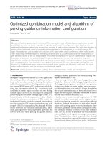
Figure 1: System overview.
resilience—features included in H.264/AVC for this purpose
are discussed, for example, in [7].
In this work we assume that our rate adaptation entity—
referred to as scheduler—has sufficient information and in-
telligence to be able to drop packets with respect to their rela-
tive importance. A formalized framework under the acronym
rate-distortion optimized packet scheduling has been intro-
duced [8] and serves as the basis for several subsequent pub-
lications. Obviously, this strategy requires a regular syntax,
that is, by defining more and less important packets in a
stream. Hence, if bit rate variations on the transmission path
are expected, it is wise to preencode media streams with ap-
propriate packet dependencies, such that the importance of
the packets in the stream can be easily differentiated by the
network components. The H.264/AVC standard already of-

fers some options to support packets with different impor-
tance for bit rate adaptivit y. However, a scalable extension,
which will also include classical SNR-scalability, is still under
discussion [9] and will not be considered here. Our proposed
streaming system will thus rely on three different means for
bit rate adaptivity, namely, (i) play out buffering, (ii) tempo-
ral scalability, and (iii) advanced bit stream switching.
The remainder of this paper is structured as follows: we
will start with a brief overview of an end-to-end wireless
video streaming system in Section 2. Next, we wil l introduce
the various features available in H.264/AVC to support tem-
poral scalability and bit stream switching in Section 3.We
will present suitable encoding solutions for these features and
develop an abstract framework for describing video stream-
ing over arbitrary VBR channels. Section 4 then deals with
a specific class of VBR channels, which result from includ-
ing a wireless link in the end-to-end transmission chain. We
will discuss several mathematically tractable models of differ-
ent complexity to describe the influence of wireless links on
packet transmission. For the system considered in this work,
namely EGPRS, we will propose a relatively simple, yet suf-
ficiently accurate description of the channel characteristics.
In Section 5, we will integrate the previously developed con-
cepts into an optimized decision making strateg y for the se-
lection of frames and versions in a wireless streaming sce-
nario. Experimental results for H.264/AVC video streaming
over EGPRS links wil l demonstrate the applicability of our
strategy in Section 6. The paper concludes with some general
remarks and a summary of future work topics.
2. SYSTEM OVERVIEW

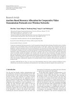
Figure 1 shows a simplified wireless streaming system, which
usually consists of an end-to-end connection between a me-
dia streaming server and a client. The latter requests preen-
coded data stored at the server to be streamed to the end user.
The client buffers the incoming data and starts with decoding
and presentation of the reconstructed video sequence after
some initial delay. Once playback has started, a continuous
presentation of the sequence should be guaranteed. For CBR
channels with constant delay successful play out can be guar-
anteed by encoding and streaming of the video sequence such
that the resulting bit stream contains a leaky bucket [10].
However, in our investigated system neither the bit rate
nor the delay is constant, and some data units are not even
available at the decoder. Therefore, the media streams stored
at the server have to be not only compression efficient, it
should also be possible to flexibly adapt their bit rate to vary-
ing conditions on the wireless link.
H.264/AVC, in addition to its compression efficiency, also
provides means for bit rate adaptivity: the flexible reference
frame concept in combination with generalized B-pictures
allows a huge flexibility on frame dependencies, which can b e
exploited for temporal scalability and rate shaping of preen-
coded video. For example, the rate can easily be adapted by
dropping nonreference frames, which does not result in error
propagation. This H.264/AVC operation mode is equivalent
to temporal scalability. Furthermore, sequences could be en-
coded such that, for example, less important background is
dropped in favor of a more important foreground scene [11].
However, very often it is still necessary to further adapt the
bit rate in the application, usually in larger bit rate scales, as

well as in time scales larger than the initial play out delay. In
Thomas Stockhammer et al. 3
Version 1
0
I
1
P
2
P
3
P
4
P
5
P
6
P
SSP
Version 2
SP SP
(a)
Version 1
0
I
1
P
2
P
3
P

4
P
5
P
6
P
SI
Version 2
SP SP
(b)
Figure 2: Bit stream switching w ith SP- and SI-pictures in H.264.
this respect, it has been recognized that the bit rate on wire-
less links is a precious resource, especially when compared
to storage on servers. Finally, most applications provide suf-
ficient buffer feedback, as well as channel state information,
such that the streaming server has at least an estimate of the
supported bit rate. Under these common premises bit stream
switching provides a simple, yet powerful, means to support
bit rate adaptivity in wireless streaming environments. In this
case the streaming server stores the same content encoded
with different versions in terms of rate and quality. Each of
these versions must include means to randomly switch into
it. Instantaneous decoder refresh (IDR) pictures provide this
feature, but they are also costly in terms of compression effi-
ciency (for an analysis of bit stream switching for streaming,
see [12]).
The switching predictive (SP) picture concept in H.264/
AVC [13], however, is more adequate for this purpose: in this
case the streaming server not only stores different versions of
the same content, but also secondary SP-pictures, as well as

SI-pictures. As long as the bit rate does not change, efficient
primary SP-pictures are transmitted at the pre-selected pos-
sible switching points. If switching becomes necessary, one
can rely on secondary SP- or SI-pictures. Some preliminary
work on bit stream switching using the SP-picture concept
for congested links has been presented in [14].
In Figure 2, a simplified switching scenario is depicted
with only two preencoded versions 1 and 2. An extension
to more than two versions is straightforward, but is omitted
here for the sake of clarity. These two versions result from en-
coding of the same original video sequence with two differ-
ent quantization parameters. Primary SP-pictures have been
used periodically at identical positions in both sequences.
Thus, at every “SP-position” either the primar y is transmit-
ted, if no switching happens, or the secondary (either SSP or
SI) is transmitted in case of switching.
In this work we will consider a wireless video streaming
environment which employs a central unit at the transmitter,
referred to as scheduler. The latter has access to information
about all source data to be transmitted next, as well as to in-
formation on current expected transmission conditions. The
scheduler attempts to optimize its decision which packets, as
well as which versions, are to be transmitted next. The ac-
cessible source and channel information will be specified in
more detail in the following two sections, and the proposed
scheduler is presented in Section 5.
3. A FRAMEWORK FOR VBR STREAMING
OF H.264/AVC VIDEO
3.1. Preliminaries of the SP-picture concept
The SP-picture concept allows applying predictive coding

even in case of different r eference signals by performing the
motion-compensated prediction (MCP) process in the trans-
form domain rather than in the spatial domain. The ref-
erence frame is quantized—usually with a finer quantizer
than that used for the original frame—before it is forwarded
to the reference frame buffer. The resulting so-called pri-
mary SP-pictures are placed in the encoded bit stream at the
pre-selected possible switching points. In general, they are
slightly less compression-efficient than regular P-pictures,
but significantly more efficient than regular IDR-pictures.
The major benefit results from the fact that the quantized ref-
erence signal can be generated mismatch-free using any other
prediction signal. In case that this reference signal is gener-
ated by predictive coding, the picture is referred to as sec-
ondary SP (SSP) picture. They are usually significantly less
efficient than P-pictures, as an exact reconstruction is nec-
essary. To generate the reference signal without any previ-
ous dependencies, the so-called switching-intra (SI) pictures
can also be used, which are only slightly less inefficient than
common I-pictures, but can also be used for adaptive error
resilience purposes. For more details on this unique feature
within H.264/AVC the interested reader is referred to [13].
3.2. An optimized encoder for SSP/SI-pictures
An encoder realization for generating primary SP-pictures is
already included in the H.264/AVC test model software. In
addition, we have developed an optimized encoder for SSP-
pictures, as well as for SI-pictures. The respective encoder
structure for SSP-pictures is shown in Figure 3.Here,lower-
case letters (e.g., l) denote quantized signals, while capital let-
ters (e.g., L) denote nonquantized signals. Furthermore, sig-

nals in the transform domain are indicated by the letter “l,”
while signals in the pixel domain are indicated by the letter
4 EURASIP Journal on Applied Signal Processing
l
err
Inv. quant
QPSP
L
err
+
L
rec
Quant
QPSP2
l
rec
Inv. quant
QPSP2
L
rec
Decoding of
source stream 1
Inv. trans
F
rec
Decoded frame
Frame
memory
Trans
L

pred
Inter-
prediction
Reference frame(s) F
ref,1
Entropy decoding and demultiplexing
Optimized
prediction &
mode decision
L
pred,1
Quant
QPSP2
l
pred,1
+
+
l
err,1-2
F
rec,2
l
rec,2
Encoding of
switching stream 1-2
Bit stream
SSP
1-2
Entropy encoding
Modes,

motion data
l
err
Inv. quant
QPSP
L
err
+
L
rec
Quant
QPSP2
l
rec
Inv. quant
QPSP2
L
rec
Decoding of
target stream 2
Inv. trans
F
rec
Decoded frame
Frame
memory
Trans
L
pred
Inter-

prediction
Motion vectors
and mode info
Entropy decoding and demultiplexing
Figure 3: Optimized secondary SP-picture encoder.
Thomas Stockhammer et al. 5
“ f .” The individual meaning of a signal (e.g., pred for “pre-
dicted”) can be derived from its index.
According to Figure 3 we obtain the SSP-picture for
switching from source stream 1 to target stream 2 by extract-
ing and combining information from both runs. T he encod-
ing process for the secondary representations depends on the
signal l
rec,2
that is generated in the encoding and decoding
process of the primary target SP-picture. We decided to use
the decoding process of target stream 2 for exporting l
rec,2
as shown in Figure 3. SSP-encoding also requires the predic-
tion signal L
pred,1
. In our implementation, L
pred,1
is generated
using all reference frames F
ref,1
, which are available by de-
coding source stream 1. For SI-pictures the same concept ap-
plies with the only difference that the prediction signal can
be computed w ithout any signals exported from stream 1.

It is also worth mentioning that the straightforward ap-
proach to simply use the prediction signal, motion vec-
tors, and modes from encoding/decoding the primary source
stream 1 is not efficient: the partition modes and the motion
vectors chosen for encoding the source primary SP-picture
do not necessarily fit well for encoding the SSP and result
in a suboptimal prediction signal with a large prediction er-
ror l
err,1 2
. This implies that coding efficiency is low, as the
residual has to be encoded without any further quantization.
Hence, a prediction signal L
pred,1
is required which minimizes
the residual. Since no restrictions apply on L
pred,1
,wecanop-
timize it by using all available reference frames F
ref,1
. Classi-
cal rate-distortion optimization [15], as used in the JM test
model, is applied. However, the encoded SSP will be iden-
tical to the primary SP-reconstruction of the target stream.
The goal of the motion estimation and compensation must
therefore be to match the reconstructed primar y target frame
F
rec,2
, rather than the original frame F
orig
. With this modified

mode selection we save up to 10% in bits for SSP-picture cod-
ing compared to the case when we use the prediction signal
optimized to F
orig
. The gains compared to the nonoptimized
approach using the prediction signal L
pred,1
, for which the
frame sizes often exceed or equal those for SI-pictures, are
in the order of 100–400%. For details on encoding results,
the exact encoder implementation, as well as on guidelines
for the selection of quantization parameters for primary and
secondary representations, we refer to [14, 16].
3.3. General abstraction of the encoding, transmission,
and decoding processes
Efficient streaming media algorithms require a formalized
description of the encoded multimedia data to be able to
make good decisions during the transmission process [8].
Assume that source units f
n
, n = 1, , N (i.e., video frames),
are encoded and mapped one-to-one onto data units P
n
(i.e.,
packets). Any advanced packetization modes, such as flexible
macroblock ordering, slice structured coding, or packet in-
terleaving schemes, are not considered here. Note, however,
that our framework is general enough to include such con-
cepts. In addition, we assume that for each source unit f
n

we
generate several versions v
= 1, , V, which are represented
by individual data units P
n,v
. The reconstructed version of
each source unit is denoted as

f
n,v
. Furthermore, we define
a quality measure Q( f ,

f ) reflecting the rewards/costs when
representing f by

f .
Each source unit (and hence each data unit) has assigned
a decoding time stamp (DTS) T
n
representing the latest time
instant the data unit P
n
must be decoded to be useful. The
decoding time is relative to T
1
, which is assumed to be 0 with-
out loss of generality. Data unit indices are ordered with in-
creasing DTS T
n

. According to [8], video encoding and pack-
etization can then be represented as a directed acyclic graph.
However, note that this only holds for the data units within
one version. An extended framework for different versions is
not addressed in [8]. We restrict ourselves in the following to
the practical case where the graph for each version is of iden-
tical structure. Again, generalization to different structures
for each version is straightforward, but the benefit in terms
of encoding efficiency needs to be carefully considered. To
specify decoding dependencies among data units, we write
n
n if P
n
is necessary to decode P
n
.
When transmitting a stream to a client, a server may se-
lect an appropriate version vector v
= v
n
N
n
=1
,withv
n
the
version chosen for each f
n
. Hence, with this definition any
arbitrary stream-switching strategy is possible, since differ-

ent versions may be transmitted for each successive data unit.
Ho wever, for our strategy we apply restrictions on version
vector elements to avoid the problem of reference frame mis-
matches: since switching is only allowed at I- or SP-picture
positions, versions can only change at these positions as well.
Assume now that we operate in an environment where
not necessarily all data units are received at the media de-
coder. In this case, concealment has to be done for any rep-
resentation of a missing data unit. In the remainder we ap-
ply the common “freeze-picture” concealment, that is, miss-
ing data units are represented by the timely nearest available
source unit. Note that while the encoder only considers this
type of error concealment in the optimization process, our
decoder does actually apply this strategy. The index of the
first candidate to conceal source unit f
n
is denoted by the
concealment index c(n). If there is no preceding source unit,
for example, I-pictures, we assume that the lost source unit is
concealed with a standard representation, for example, a grey
image (denoted as c(n)
= 0).
In case of consecutive data unit loss, concealment is ap-
plied recursively. Assume that c(n)
= i.IfdataunitP
i
is also
lost, the algorithm uses source unit f
j
to conceal f

i
, that is,
c(i)
= j. To avoid any lengthy recursive notation we simply
use j
n to express the fact that source unit f
n
is eventually
concealed with unit f
j
. The resulting concealment dependen-
cies can also be expressed by a directed graph. Figure 4 shows
an example of possible frame dependencies and the corre-
sponding concealment graph.
3.4. Importance definition
To allow prioritization of different data units and also of
different versions over others, the importance of a single
data unit for the overall reconstruction quality needs to be
quantified. The previous definitions and the abstraction of
6 EURASIP Journal on Applied Signal Processing
I
1
P
2
P
5
I
8
B
3

B
4
B
6
B
7
B
9
B
10
(a)
G
I
1
P
2
P
5
I
8
B
3
B
4
B
6
B
7
B
9

B
10
(b)
Figure 4: Frame dependencies and concealment graph.
the encoding, transmission, and decoding processes lead to
the definition of the so-called importance of each data unit
P
n,v
: the latter reflects the amount by which the quality at the
receiver increases if the data unit is correctly decoded and can
be written as
I
n,v

1
N
⎛
⎜
⎜
⎝
Q

f
n
,

f
n,v

Q


f
n
,

f
c(n),v

+
N

i=n+1
n
i

Q

f
i
,

f
n,v

Q

f
i
,


f
c(n),v

⎞
⎟
⎟
⎠
.
(1)
The importance definition takes into consideration the
quality of data unit P
n,v
, the chosen concealment strategy,
as well as the dependency and concealment graph. In other
words, the importance quantifies the improvement in quality
if the source unit contained in P
n,v
is displayed instead of
the concealment source unit f
c(n),v
forthisunit,aswellas
for all other source units for which f
n
is eventually used for
concealment.
3.5. Received and expected quality
The end-to-end performance of a streaming media system
strongly depends on the versions chosen (expressed by the
version vector v) and the amount and importance of packets
not available at the decoder. To be more specific, we define

the observed channel behavior at a streaming client for data
unit P
n,v
as c
n
 1 {data unit P
n,v
available}.Here,1 A de-
notes the indicator function being 1, if A is true, and 0 oth-
erwise. Hence, the combination of a certain observed chan-
nel sequence c
= c
1
, , c
N
with (1) and the concealment
strategy as introduced above yields the following expression
for the (actual) received quality:
Q(c, v)  Q
0
+
N

n=1
I
n,v
n
c
n
n

1

m=1
m
n
c
m
. (2)
Here, Q
0
 (1/N)

N
n
=1
Q( f
n
,

f
0
) denotes the minimum
quality, if instead of the original sequence all pictures are
presented as grey. The latter is obviously quite hypothetical,
but it is necessary to have a comprehensive framework. In
summary, in order to benefit from data unit P
n
,itisneces-
sary that all data units P
m

it depends on are also available
at the receiver. For a proof that (2) actually corresponds to
the received quality given the above assumptions, we refer to
Appendix A.
The importance of each data unit and version is quite eas-
ily computed during the encoding process. As a consequence,
(2) significantly simplifies the simulation of video stream-
ing systems, as the achievable quality at the simulated me-
dia clients can be determined via linear combination of the
channel vector and the importance of the selected versions of
each data unit. Any decoding of erroneous video streams is
thus not necessary.
The practical importance of (2) for system optimization,
however, is ra ther limited, since in wireless transmission sys-
tems, the channel behavior is in general not deterministic.
Nevertheless, the notion of importance can be used quite ef-
fectively at the transmitter for simple computation of the ex-
pected quality (at the receiver), as will be shown in the fol-
lowing: a certain data unit might be lost entirely or might
arrive too late at the receiver such that the decoding of the
data unit is no more useful due to expired deadlines (we as-
sume here that the client does not u se any advanced strate-
gies,suchasrebuffering). The channel behavior sequence
C 
C
1
, , C
N
is in general random, with C
n

0, 1 the
random variable indicating w h ether data unit n is received
successfully (C
n
= 1) or lost (C
n
= 0). Therefore, not only the
channel is random, but also the received quality, denoted as
Q(C): for certain channel realizations we obtain a good qual-
ity, whereas for others the received quality is much worse.
In the following we are interested in a single measure to
compare the different transmission strategies. The most ob-
vious and suitable measure is the expected quality E
Q(C) .
The following equation provides a definition of the expected
received quality, as well as a simplified method to derive it:
E

Q(C)



c 0,1
N
Q(c)Pr C = c
= Q
0
+
N


n=1
I
n
Pr

C
n
= 1
k n
C
k
= 1

n 1

m=1
m
n
Pr

C
m
= 1
k m
C
k
= 1

=
Q

0
+
N

n=1
I
n
Pr

C
n
= 1
k n
Δ
k
= 1

.
(3)
Note that the expectation in this case is only over the channel
statistics C. For a proof of the various equalities in (3), we
refer to Appendix B.
Thomas Stockhammer et al. 7
3.6. Summary: media abstraction for video
streaming over VBR channels
With these preliminaries we are able to develop an effective
abstract ion of streamed media data. For channels which ex-
hibit data unit loss (as will be considered in the remainder
of this work), it is sufficient to know the number of encoded
source versions V, the initial quality Q

0
, and the following
metrics for each data unit n
= 1, , N and each version
v
= 1, , V:
(i) the importance I
n,v
,
(ii) the data unit size R
n,v
in bytes,
(iii) the decoding time stamp T
n
,and
(iv) the dependencies expressed by the index of the directly
preceding data unit(s) of P
n
.
Furthermore, for each SP-picture in each version v, the data
unit size R
n,v v
of the SSP-picture when switching to ver-
sion v
and the SI-picture size are required [16]. As already
mentioned, this abstract description can be used on the one
hand to effectively simulate video streaming over lossy chan-
nels (via (2)). On the other hand, (3) or one of its variants
provides a means to optimize the transmission schedule, as
will be shown in Section 5.

4. A FRAMEWORK FOR THE DESCRIPTION
OF WIRELESS LINKS
4.1. General characteristics and modeling aspects
Wireless channels are becoming increasingly important as
a transport medium for various types of multimedia in-
formation. While the appeal of tetherless mobility is great,
numerous issues need to be resolved in order for wireless
transport of real-time multimedia data to become reality
(including communications issues, low-power implementa-
tions, etc.). In this work we consider a scenario where due
to the user’s mobility the channel behavior will be inherently
time-varying, with periods of higher data rates alternating
with periods of lower rates.
In general, the available bandwidth and, therefore, the
bit rate over the radio link are limited. In addition, the
mobile environment is characterized by harsh transmission
conditions in terms of attenuation, shadowing, fading, and
multiuser interference, which result in time- and location-
dependent channel conditions. New directions in the design
of wireless systems do not necessarily attempt to minimize
the error rates in the system, but to maximize the system
throughput. This is especially attractive for services with re-
laxed delay constraints, such as file downloads and stream-
ing applications. The nonergodic behavior of the channel is
exploited such that in case of good channel states a signif-
icantly higher data rate is supported than in bad channel
states. This behavior is typically achieved by rate adaptation
via adaptive modulation and coding (AMC). In addition, re-
liable link layer protocols with persistent automatic repeat re-
quest (ARQ) are often used to guarantee error-free delivery.

This concept is, for example, applied in EGPRS and further
extended in high-speed downlink packet access (HSDPA). In
the following we will focus on EGPRS, since both appro-
priate descriptions and models are available. However, most
concepts discussed and presented here are also applicable in
other wireless systems with slight modifications and param-
eter adjustments.
In order to emulate time-varying EDGE-(enhanced data
rates for GSM evolution) based radio channels in real time,
a model has been developed and proposed in [17], which al-
lows describing both short-term and long-term effects. This
simulation model consists of three levels, which reflect typi-
cal physical layer and system properties [17].
(i) The top level of the simulation model considers the
overall cellular layout. Users are distinguished in two
groups, one in good locations, and one w ith poorer
receiving conditions.
(ii) The second level characterizes system configurations,
such as the applied power control, the velocity of the
user, the interference conditions, and other system dy-
namics. This is reflected in the model by defining sev-
eral states, which basically correspond to the coding
schemes defined for EGPRS.
(iii) Finally, the lowest level specifies the transmission con-
ditions in a certain state. Throughout this work we as-
sume a static resource allocation in terms of a constant
number of assigned radio slots α. Independent of the
current state, link layer packets are sent out periodi-
cally according to the fixed transmission time interval
(TTI) τ

I
. The payload size C
ξ
of the packets differs for
each state ξ,asdifferent channel code rates and modu-
lation schemes are applied to adapt to changing trans-
mission conditions. Furthermore, since we assume op-
eration in persistent acknowledged mode (i.e., lost link
layer packets are retransmitted until they are received
correctly), we extend the channel model to incorporate
the transmission mode.
We summarize the description of the channel model in-
cluding persistent acknowledged mode for a certain state ξ
as W
ξ
 W (C
ξ
, τ
I
, p
ξ
, N
τ
), with p
ξ
the loss probability, and
N
τ
the number of transmissions in state ξ.Incaseofmul-
tislot transmission and noise-limited scenarios, the payload

is multiplied with α, such that C
ξ
αC
ξ
. In interference-
limited scenarios, the TTI can be divided by the number of
slots, that is, τ
I
τ
I
/α.
Figure 5 depicts the statistical EDGE radio link model
specified by a two-group, five-state Markov chain according
to [17]. The radio system is completely characterized by the
payload size C
ξ
for each state, the link layer packet error rate
1
p
ξ
= p, the state transition probabilities λ, μ
1
,andμ
2
,and
finally, the group probabilities p
G,1
and p
G,2
. All of these pa-

rameters depend on the actual radio system configuration,
such as frequency reuse pattern, power control option, num-
berofuserspersector,andsoforth.Anexemplarysetof
1
For the investigated EGPRS configuration the link layer packet error rate
is independent of the state. In other words, the coding schemes and the
power are adapted such that a constant error rate is maintained.
8 EURASIP Journal on Applied Signal Processing
Group 1
S
0
1 λ
μ
1
λ
1
μ
1
λ
S
1
μ
1
λ
S
2
1 μ
1
(a)
Group 2

S
3
1 λ
μ
2
λ
S
4
1 μ
2
(b)
Figure 5: Two-group, five-state Markov channel model.
Table 1: Radio system parameters for EGPRS with frequency hop-
ping, frequency reuse 1/3, and radio aware power control.
Users/sector p
G,2
λμ
1
μ
2
p
20.93 0.30.055 0.05 0.11
80.64 0.30.094 0.30.20
15 0.28 0.30.27 0.59 0.27
parameters [17] for the EDGE radio system used in this work
is presented in Ta ble 1.
4.2. Abstract channel representation
An accurate model as presented in Section 4.1 is definitely
helpful to obtain representative results. However, it is ob-
vious that such a model is never comprehensive, nor can it

be assumed that the parameters are known in advance. Nev-
ertheless, it is always advantageous to include channel state
information into decisions at the transmitter. Therefore, an
abstraction of the previously introduced channel character-
istics to some meaningful but also measurable and simple in-
formation at the sender unit is highly desired.
Sufficient information for our scheduling entity (speci-
fiedinmoredetailinSection 5) is some a priori information
on the probability that the channel supports a certain data
rate over a certain time interval. More precisely, we ask how
likely it is that a certain amount of data has left the sender
buffer by some time measured as delta from the actual time
τ
a
. Note that in our case the sender and the receiver buffers
are each other’s complement and we assume the propagation
delay to be negligible. Hence, without loss of generality, the
time the data leaves the sender buffer is equivalent to the time
it is available at the receiver. To formalize this notion, we de-
fine the event that the channel is able to support some rate
r (in bits) within a time interval t as R(r, t). However, it is
not only sufficient to receive a certain rate by some time for
the data to be useful at the receiver: due to the dependency
graph it might be necessary that also some preceding data is
sent out at some earlier time. Therefore, we generally require
a joint probability distribution Pr

i
R(r
i

, t
i
) ξ , which de-
pends on the probability of the joint events, as well as on the
current channel state ξ at time τ
a
.
Whereas access to an estimate of the single event success
probability Pr
R(r, t) is feasible, as will be shown later, es-
timation of the joint probability function is r ather complex.
However, if we only have access to the single event success
probabilities, the joint event success probability can at least
be bounded by the product of the single success probabilities
and the minimum of the single success probabilities, that is,

i
Pr

R

r
i
, t
i

Pr


i

R

r
i
, t
i


min
i

Pr

R

r
i
, t
i

.
(4)
4.3. Simplified description for EGPRS
The exact derivation of the single event success probability
distribution for complex channel models is still too com-
plicated and likely without practical relevance, as discussed
previously. Therefore, we attempt to obtain a simplified de-
scription for the single event success probability Pr
R(r, t)
in case of an EGPRS channel. Despite being verified only for

this specific system, it can be conjectured that the proposed
model is relatively generic and can also be adapted for other
wireless systems.
Recall that transmission within each single state is repre-
sented by W (C
ξ
, τ, p
ξ
, N
τ
). Then, let X
ξ
be a random variable
which describes the amount of data transmitted with a single
link layer packet in state ξ,withX
ξ
0; C
ξ
. Furthermore,
let 1
p be the probability of successful packet reception
(X
ξ
= C
ξ
), and p the probability of a packet loss (X
ξ
= 0).
The mean and variance of this process are m
ξ

= C
ξ
(1 p
ξ
)
and σ
2
ξ
= C
2
ξ
(1 p
ξ
)p
ξ
,respectively.
As, in general, provision of feedback and retransmission
at the link layer happen quite fast, the respective delay can be
neglected. This is especially the case for scenarios where the
channel propagation time of one packet is sufficiently smaller
than the time interval between two consecutive higher-layer
data units. Moreover, in delayed feedback systems packet la-
beling allows reordering of received packets. Therefore, we
can assume that the lost packet will immediately be retrans-
mitted at time instant k + 1. Then, for some channel state
sequence ξ
K
= ξ
1
, , ξ

K
, the random sum rate S(ξ
K
)can
be defined as
S

ξ
K


K

k=1
X
ξ
k
=
N
ξ

ξ=1
ω
ξ
X
ξ
,(5)
with ω
ξ
the frequency of state ξ in the sequence ξ

K
.Forsuffi-
ciently large K, it can be assumed that the sum rate S(ξ
K
)ap-
proaches a normal distribution due to the central limit theo-
rem [18]. In addition, if the frequency ω
ξ
for each state is also
Thomas Stockhammer et al. 9
sufficiently large, the distribution of the normalized sum rate
can be characterized as a normal distribution,
2
that is,
S

ξ
K

Km

ξ
K

σ

ξ
K

K

N (0, 1), (6)
with normalized mean
m

ξ
K

=
1
K
N
ξ

ξ=1
ω
ξ
m
ξ
(7)
and normalized variance
σ
2

ξ
K

=
1
K
N

ξ

ξ=1
ω
ξ
σ
2
ξ
(8)
due to the central limit theorem and some extensions [18].
However, in general the state sequence is also random
and follows the underlying Markov model. Assuming that
the actual state ξ is known, we are interested in the distri-
bution of the sum rate S
K ξ
after the transmission attempt of
K link layer packets, that is,
S
K ξ

K

k=1
X
ξ
k
ξ
. (9)
For K sufficiently large, a normal distribution of the sum
rate is still justified. However, the derivation of the mean and

the variance is not straightforward. Therefore, it is recom-
mended to estimate those parameters m
K ξ
and σ
2
K
ξ
depend-
ing on the number of link layer packets K and the initial state
ξ. If the channel state, however, is not accessible, we denote
the mean as m
K
and the variance as σ
2
K
. Figure 6 shows the
normalized means m
K ξ
/K and m
K
/K, as well as the nor mal-
ized variances σ
2
K
ξ
/K and σ
2
K
/K for the EGPRS parameters
given in Tabl e 1 . When comparing the different curves for

the two parameters, it is obvious that additional simplifica-
tions and modeling might be performed. In a practical sys-
tem, these parameters might be estimated in advance or are
constantly updated during the transmission. In the following
we will assume that the parameters m
K ξ
and σ
2
K
ξ
,oratleast
some estimates, are available to the transmitter.
With knowledge of the mean and the variance for each K
(and each initial state ξ), the probability of a certain sum rate
is readily expressed as
Pr

S
K
= s

=
1

2πσ
2
K
e
(s m
K

)
2
/2σ
2
K
. (10)
Hence, the single event success probability in case of knowl-
edge of the channel state can be written as
Pr

R(r, t)

=
Pr

S
t/τ
3
r

=
1
2
erfc

r m
t/τ
3
2σ
t/τ

3

. (11)
For ease of exposition, we will in the following only present
the case where the channel state is not known. The exten-
2
Throughout this work, N (m, σ
2
) will denote the normal distribution
with mean m and variance σ
2
.
0 50 100 150 200 250 300
K
100
200
300
400
500
600
700
800
900
m
K
(ξ)/K
m
K
(ξ = 1)
m

K
(ξ = 2)
m
K
(ξ = 3)
m
K,1
m
K
(ξ = 4)
m
K
(ξ = 5)
m
K,2
(a)
0 50 100 150 200 250 300
K
100
200
300
400
500
600
700
800
900
σ
2
K

(ξ)/K
σ
2
K
(ξ = 1)
σ
2
K
(ξ = 2)
σ
2
K
(ξ = 3)
σ
2
(b)
Figure 6: Normalized m
K ξ
/K and m
K
/K as well as normalized vari-
ances σ
2
K
ξ
/K and σ
2
K
/K versus number of link layer packets K.
sion to the case when the channel state is known, however, is

straightforward.
5. OPTIMIZED TRANSMISSION SCHEDULING
AND BIT STREAM SWITCHING
5.1. Transmitter assumptions
We will consider a wireless v ideo streaming system as in-
troduced in Section 2, with a central scheduling unit in the
transmitter. The latter should decide at each time instant
10 EURASIP Journal on Applied Signal Processing
which data unit to transmit next out of the set of available
ones
P
n,v
,withN = 1, , N and v = 1, , V , on the
streaming server. To achieve good user experience, some ob-
vious principles for the selection of data units are as follows.
(1) The algorithm should be able to react to varying chan-
nel conditions by bit stream switching. Only if the
channel conditions change too fast, additional reduc-
tion of the temporal resolution should be allowed.
(2) Data units should be transmitted as close as possible to
the time instant they are due at the receiver. Otherwise,
bandwidth is wasted, which might result in expiration
and consequently dropping of other earlier data units.
(3) Nevertheless, it should be possible to transmit impor-
tant data units earlier to guarantee their delivery even
in bad channel conditions.
(4) Version switching should preferably be accomplished
with SP-frames rather than with SI-fr ames.
Previous work on this subject has for example been per-
formed in [6], which is an extension to the well-known early

deadline first (EDF) scheduling [5]. In [6] the EDF schedul-
ing is extended taking into account frame dependencies. In
this work we formalize the concept of frame dependencies
and frame importance, extend it to stream switching, and in-
troduce schedulers which try to optimize sending order. Be-
fore we present our proposed algorithm for optimized trans-
mission scheduling and bit stream switching, we want to dis-
cuss some reasonable constraints. The latter will be helpful
for significantly reducing the amount of possible data units
to be considered in the optimization process.
(i) Each data unit P
n,v
is only transmitted once from end-
to-end, since we a ssume that the lower link layer re-
transmission protocol clears out all errors. Hence, a
loss in our system only happens due to late-arrival at
the media client.
(ii) If the transmission of data unit P
n,v
in version v has
been attempted, all data units at the same position n in
the video sequence, which resemble different versions
v
= v, are removed from the set of data units consid-
ered for future transmissions.
(iii) It is also assumed that the information on the success-
ful reception or loss of a single data unit is immedi-
ately available at the transmitter. As a consequence, a
status
3

γ
n
can be assigned at the t ransmitter to each
position n in the video sequence. If any data unit P
n,v
(v = 1, , V) has already been transmitted, the status
takes on one of the following two (final) values:
– γ
n
= ACK, if the data unit is known to have been
received correctly and
– γ
n
= NAK, if the data unit is known to be lost.
(iv) Positions a t which no data unit P
n,v
(of any version)
has been transmitted yet are assigned one of the re-
maining two ( intermediate) status values:
3
Note that the status is only indexed with the position n, but not with the
version v.
– γ
n
= R (for READY), if transmission is possible
in general, since all ancestors P
n ,v
n
are available
at the receiver (i.e., have γ

n
= ACK),
– γ
n
= P (for PENDING) if transmission is not
recommended yet, since there are still some miss-
ing ancestors at the receiver (i.e., which have
γ
n
= P).
(v) As a consequence, only data units with status γ
n
= R
are considered for transmission.
(vi) Any data units P
n,v
with expired deadline T
n
+ Δ >τ
a
(with Δ the initial play out delay and τ
a
the actual time
at the transmitter) are not transmitted and, together
with all of their dependants, are assigned γ
n
= NAK.
Note that this procedure is already quite intelligent, as
in this case the channel is not blocked with no more
useful data.

(vii) Switching positions in the video sequence are assigned
two status values: one for SI-frames γ
n
and one for SP-
frames
γ
n
. For SP-frames to be decodable, it is assumed
that it is necessary and sufficient that the previous P-
frame of any version is available.
5.2. Periodic update of side information at
the transmitter
Any optimal scheduling strategy requires up-to-date side in-
formation on the state of the system in the decision process.
Therefore, we will explain the various update steps next that
are performed before each scheduling process starts. Upon
initialization, the first position n
= 1 in the video sequence,
as well as all other switching positions which have an SI-
frame available, are assigned γ
n
= R. All other positions are
initialized with γ
n
= P. After each successful or nonsuccessful
completion of the transmission of a data unit P
n,v
n
at actual
time τ

a
, the status values at other data unit positions in the
transmitter are updated as follows.
(1) All data unit positions n
for which the deadline has
expired, that is, where T
n
+ Δ >τ
a
, are assigned γ
n
=
NAK.
(2) If the previous transmission of data unit P
n,v
n
was suc-
cessful, the corresponding status value is changed to
γ
n
= ACK.
(3) If the previous transmission, however, was not suc-
cessful, the corresponding status value is changed to
γ
n
= NAK.
(4) All data unit positions
n for which at least one ancestor
n n has status γ
n

= NAK are also assigned status
γ
n
= NAK.
(5) All data unit positions with status γ
n
= P for which all
ancestors have γ
n
= ACK are switched to status γ
n
=
R.
(6) At switching positions for which all ancestors of the
SP-frame are now available at the receiver, the status is
changed to
γ
n
= ACK. In this case, either the SI-frame
or the SP-frame (depending on the rate) for each ver-
sion can be selected as a possible candidate for trans-
mission.
Thomas Stockhammer et al. 11
After this update procedure has been performed, a new
data unit with γ
n
= R must be selected for transmission by
the scheduler a s described in the next section.
5.3. The scheduling process
The task of the scheduler is to determine an optimal trans-

mission order and version of the sent data units, which maxi-
mizes the expected overall system performance. In particular,
the scheduler decides at each transmission opportunity
(i) which data unit to transmit next, possibly out of de-
coding order,
(ii) and in case of an SP-, SI-, or I-picture, which version
to transmit next.
During this decision process the scheduler should take
into account as much side information as possible: the cur-
rently expected channel behavior, the ac tual time τ
a
,aswell
as the deadlines, the importance, the different versions, and
the updated status of different data units.
As already mentioned, the scheduler might decide to
transmit more “important” data units earlier to guarantee
their timely delivery with high probability, whereas other
data units with very low importance might not be trans-
mitted at all. Hence, we express the actual delivery order by
the transmission schedule π
= (π
1
, π
2
, ), where π
k
holds
the index of the data unit (i.e., the position in the video se-
quence) to be transmitted at (temporal) position k. Further-
more, for each element in the t ransmission schedule, a ver-

sion v
π
k
is also selected.
4
We propose to select the next data unit for transmission
based on some utility function, for which we use the expected
quality at the receiver Q(π, v). This metric generally depends
on all relevant source and channel information, such as rates,
deadlines, importance vector, a nd so forth. More specifically,
the optimal schedule π
opt
and the optimal version vector v
opt
satisfy

π
opt
, v
opt

=
arg max
(π,v)

Q(π, v), (12)
with

Q(π, v) = Q
0

+
N

n=1
γ
n
=ACK
I
n,v
n
+
N

n=1
γ
n
=NAK
0
+
N

n=1
γ
n
R,P
I
n,v
n

P

n
(π, v)
n 1

m=1
m
n

P
m
(π, v).
(13)
Here,

P
n
(π, v) expresses the probability that data unit
P
n,v
n
will be received in time for this selection of π and v.
Note that for data units with γ
n
= ACK, this probability
is equal to 1, while for γ
n
= NAK it is equal to 0. In case
4
Note that the version vector v = v
n

N
n
=1
is ordered with respect to the
position of the data units in the video sequence.
γ
n
R, P , the probability depends on the sum rate of the
scheduled data units, the delivery deadline T
n
+ Δ, the actual
time τ
a
, and the channel statistics R(r, t), and can be written
as

P
n
(π, v) = Pr

R

ρ
n

k=1
R
π
k
,v

π
k
T
n
+ Δ τ
a


m n
γ
m
R,P
R

ρ
m

k=1
R
π
k
,v
π
k
T
m
+ Δ τ
a

, π, v


,
(14)
where ρ
n
defines the (temporal) position of data unit P
n,v
n
in
the schedule π.
Hence, when determining the expected quality according
to (14), we acknowledge the fact that due to the dependencies
in the video sequence not only the actual data unit must have
been received, but also all of its predecessors. The above nota-
tion can be s implified by using the joint probability P
n
(π, v)
instead of the conditional probability

P
n
(π, v), that is,
P
n
(π, v) = Pr
⎧
⎪
⎪
⎨
⎪

⎪
⎩

m n
γ
m
R,P
R

ρ
m

k=1
R
π
k
,v
π
k
T
m
+ Δ τ
a

π, v
⎫
⎪
⎪
⎬
⎪

⎪
⎭
.
(15)
The optimal transmission schedule and version vector
now have to satisfy

π
opt
, v
opt

= arg max
(π,v)
Q(π, v), (16)
with
Q(π, v) 
N

n=1
γ
n
R,P
I
n,v
n
P
n
(π, v). (17)
Note that in (17), we have already considered the fact that

only data units with status γ
n
= R or γ
n
= P must be part of
the schedule π. The version vector v remains identical to the
previous definition.
With these preliminaries, the scheduler repeats the fol-
lowing operations, until there are no more ready or pending
data units at the transmitter.
(1) After successful or nonsuccessful completion of the
transmission of a data unit, the status of the data
units in the transmission set is updated according to
Section 5.2.
(2) Then, by combining this updated status information
with (possibly new) channel state information, the
scheduler determines (π
opt
, v
opt
) according to (16).
(3) Finally, transmission of data unit P
π
opt,1
,v
opt,π
opt,1
is initi-
ated.
5.4. Implementation aspects and complexity reduction

The number of possible combinations the scheduler has to
compare in (16) is huge, since exchange of a single element
12 EURASIP Journal on Applied Signal Processing
in π even at some later position generally influences the ex-
pected quality and thus the selection of the next data unit.
To find the optimal schedule and version vector, in principle,
a brute-force search is necessary. Since this is far from being
practically feasible, complexity reduction is essential. In the
following we will discuss some simplifications first before we
present our optimized scheduling algor ithm.
5.4.1. Weighted cumulative importance
A major problem in the computation of the expected quality
for a certain combination
π, v originates from the fact that
all later parts in the transmission schedule can be reordered
in many ways. However, only the (typically few) data units
with status γ
n
= R are candidates for transmission, and we
want to find the best transmission order and version for them
at the actual scheduling opportunity. While the aforemen-
tioned later parts are not used, any modifications there usu-
ally affect the decision of the data unit to transmit next (i.e.,
the one we are actually interested in). Hence, we still have
to consider the influence of the transmission of current data
unitsonlaterframes:itisdefinitelynotsufficient to replace
the entire set of possible transmission schedules and version
vectors in (16) by a set which only includes data units with
γ
n

= R.
We take these dependencies into account by introducing
the weighted cumulative importance of a certain data unit
P
n,v
n
. For a given transmission schedule π and version vector
v the weighted cumulative importance

I
n
(π, v)isrecursively
defined as

I
n

π, v

 I
n,v
n
+

k γ
k
=P n k
w
k


I
k

π, v

P
k
(π, v). (18)
Here, n
k means direct dependency (i.e., n is a direct an-
cestor of k), and w
n
denotes the weight of a data unit at po-
sition n in the video sequence. In case of P-frames and B-
frames we define for the sake of simplicity
w
n

⎧
⎪
⎪
⎪
⎨
⎪
⎪
⎪
⎩
1ifn is a P-frame or SP-frame,
1
2

if n is a B-frame.
(19)
This weighted cumulative importance has to be recomputed
at each scheduling opportunity for all data u nits in the trans-
mission set with γ
n
R, P .
Assume now that the version vector v is fixed. Let S
=
n γ
n
= R be the set containing all data unit positions with
status γ
n
= R. Correspondingly, S = n γ
n
= P contains
all remaining data unit positions with γ
n
= P,whicharestill
waiting for transmission. In the follow ing we will only inves-
tigate schedules, which only have elements from S in the first
positions, before any remaining ones from
S are added. Such
ascheduleisdenotedas
π(S), π(S) . Furthermore, let us
define the sum rate of all data units in S as
R
S



n S
R
n,v
n
. (20)
Thus, the weighted cumulative importance according to (18)
can be approximated by

I
n

S, π(S), v

=
I
n,v
n
+

k S
n
k
w
k
I
k,v
k
Pr
⎧

⎪
⎪
⎪
⎪
⎨
⎪
⎪
⎪
⎪
⎩

j S
j
k
R
⎛
⎜
⎝
R
S
+
ρ
j
(S)

i=1
R
π
i
, T

j
+ Δ τ
a
⎞
⎟
⎠
⎫
⎪
⎪
⎪
⎪
⎬
⎪
⎪
⎪
⎪
⎭
,
(21)
with ρ
j
(S) the (temporal) position of data unit P
j,v
j
in π(S).
To simplify the computation of the weighted cumulative
importance, we apply the upper and lower bounds according
to (4). Let us define
P
j


r, π(S)

 Pr
⎧
⎨
⎩
R
⎛
⎝
r +
ρ
j
(S)

i=1
R
π
i
, T
j
+ Δ τ
a
⎞
⎠
⎫
⎬
⎭
. (22)
Hence, a lower bound on the weighted cumulative impor-

tance in (18) is obtained as
I
n

S, π(S), v

=
I
n,v
n
+

k S
n
k
w
k
I
k

S, π(S)

P
k

R
S
, π(S)

,

(23)
which results in the following lower bound on the expected
quality in (17):
Q

π(S), π(S)

, v

=

n S
I
n

S, π(S), v

P
n

0, π(S)

.
(24)
To obtain an upper bound on the expected quality in (17)
let us recursively define a local success probability for all k
S as

P
k

 min

P
k

R
S
, π(S)

m S m k

P
m

. (25)
Hence, an upper bound on the cumulative weig hted impor-
tance in (18) can be given for any k
S
I
k

S, π(S), v

=
I
k,v
k

P
k

+

m S
k
m
I
m

S, π(S), v

, (26)
which results in the following upper bound on the expected
quality in (17):
Q

π(S), π(S), v

=

n S
⎡
⎢
⎢
⎣
I
n,v
n
P
n


0, π(S)

+

k S
n
k
I
k

S, π(S), v

⎤
⎥
⎥
⎦
.
(27)
A third method to at least estimate the quality using the
weighted cumulative importance would be ignoring the joint
Thomas Stockhammer et al. 13
channel events. The corresponding estimate of the weighted
cumulative importance results for all n
S in

I
n

S, π(S), v




k S
n
k
I
k,v
k
P
k

R
S
, π(S)

, (28)
which yields the following estimate on the expected quality
in (17):

Q

π(S), π(S), v

=

n S
I
n,v
n
P

n

0, π(S)

+

I
n

S, π(S), v

.
(29)
The advantage of using a fi xed later schedule π(
S)and
the notion of cumulative weighted importance is that the lat-
ter can be pr ecomputed before different transmission sched-
ules π(S) are tested. The specific implementation of this
computation is not discussed in further detail here, but basi-
cally in most cases the computation starts in the leaves of the
dependency graph and moves backwards to the data unit po-
sitions with status γ
n
= R. Although none of the proposed
modifications is optimal anymore due to the fixing of the
later data unit positions in π (
S), they significantly reduce the
complexity, especially, if the set S is kept small.
The number of selected data units for the set S is referred
to as look-ahead units and is denoted by N

P
in the follow-
ing. For the selection procedure, we have used two different
modes: in the first mode, called ready selection, we choose the
first N
P
data unit positions with status γ
n
= R. In the second
mode, called sequential selection, we choose the next N
P
data
unit positions, regardless of whether their status is γ
n
= R
or γ
n
= P. In this case, the presented algorithm has to be
modified slightly, as the status of data units changes due to
scheduling. It is necessary to introduce an internal variable
which keeps track of the status during the scheduling pro-
cess. Nevertheless, for both selection modes, the fixed part
of the schedule π(
S) is sequentially filled with the remaining
data units in the order of their index n.
These definitions and simplifications can be combined in
order to develop a multistage scheduling algorithm for video
streaming over VBR links. The respective flow diagram is de-
picted in Figure 7 , and the various elements will be explained
in the next sections.

5.4.2. Separation of transmission order and
version selection
Based on one of the quality metrics in (24), (27), and (29)we
select the best transmission order π(S) for each scheduling
opportunity. During this process we always operate within
the same version, that is, if a switching point is included in
π(S), the same version as used for the previous group-of-
pictures (GoP) is selected after the point. The case of version
switching is discussed separately below.
Note that despite fixing the schedule π(
S) and only using
a single version vector, all data unit positions up to the end
N would need to be considered for the computation of the
weighted cumulative importance. However, for IDR-frame
switching it is easily shown that it is sufficient to only con-
Init
source
Transmission
order
selection
Switching
point ?
Yes
No
Yes
SI-frame ?
No
No
Exchange
with SP better ?

Yes
Version
selection
Transmit
Update
source
Still
data units ?
End
Figure 7: Flow diagram of the scheduling algorithm.
sider all data unit positions up to the next nontransmitted
IDR-frame p osition. Though this is not completely accurate
in case of SP/SI-fr ames for switching, we neglect this and use
the same strategy for transmission order selection.
5.4.3. Data unit selection
In case a nonswitching position n is selected, the version v
n
of the data unit is unambiguous, as exactly for one version
the predecessors that are available at the decoder. The corre-
sponding data unit P
n,v
n
is then transmitted. In case a switch-
ing position is selected, the corresponding data unit, how-
ever, is not immediately transmitted. If the switching posi-
tion requires an SP-frame or an IDR-frame, the version se-
lection procedure as presented below is immediately invoked.
If the switching position requires an SI-frame, an alternative
proposal is made: the selected SI-frame is replaced with the
corresponding SP-frame. If this proposal yields a better met-

ric than the SI-frame, the alternative is selected. If this is not
the case, the version selection below is invoked.
5.4.4. Version selection
In addition to the local decisions on the transmission order,
whenever a switching data unit position is due for transmis-
sion, the (possibly new) version is selected based on the fol-
lowing principles: only a single data unit position, namely
the switching position, is included in S.However,insteadof
14 EURASIP Journal on Applied Signal Processing
fixing the version vector v, we evaluate the quality for all pos-
sible versions at this position. Our proposed algorithm al-
lows taking into account not only the version selection of the
next switching point, but a total of N
s
switching points. Note
that b etween two switching points the version is fi xed for all
data units to the version of the preceding switching point.
Recursive computation of the quality in (24), (27), or (29)is
then applied using the weighted cumulative importance. The
number of considered switching points N
s
is also referred to
as look-ahead switching points.
Obviously, the more switching points N
s
we take into
consideration, the more complex the algorithm gets, but the
performance also increases as more future data is taken into
account for the decisions. In the next sec tion, we will eval-
uate the performance of different system parameters and

scheduling options for our proposed scenario and optimiza-
tion strategy.
6. EXPERIMENTAL RESULTS
6.1. Simulation parameters
An exemplary set of simulations has been carried out using
the following parameters: we have encoded V
= 4 versions
ofaQCIFsequenceoflengthN
= 2698 with alternating
speakers and sport scenes using H.264/AVC test model soft-
ware JM8.2. The sequence has a length of about 90 seconds
and contains sufficiently diverse content to yield representa-
tive results. We used a single QP for each version, namely
QP
= 28, 32, 36, 40, and a common frame rate of 30 fps,
without any additional rate control algorithm. A group-of-
picture (GoP) structure with IBBPBBP SP has been applied
with SP-picture distance of 1 second. The SP-pictures have
“IDR” property in the sense that referencing over SP-pictures
is not permitted. In addition, both SSP- and SI-pictures are
possible. The initial play out delay at the streaming client is
Δ
= 1.5 seconds.
The wireless link is modeled using the EGPRS channel
model according to [17]. We restrict ourselves to the more
challenging scenarios with 8 and 15 users per cell according
to Tabl e 1 . Changes among the two groups of channel states
may happen statistically independent every 20 seconds. Each
simulation point represents the algebraic mean over 200 in-
dependent channel realizations.

As reference system, we also encoded the same video se-
quence with the rate control provided in JM8.2 to obtain
two single-rate bit streams, one with 69 kbps and one with
96 kbps. The same GoP structure was used, but I-pictures
have been applied instead of SP-pictures. We also investigate
the case where we only apply SI-frames, such that the perfor-
mance is actually similar to IDR-picture switching.
In the following we will compare the achievable perfor-
mance for different scheduler settings (i.e., in terms of dif-
ferent number of look ahead units and look ahead GoPS),
different selection modes (i.e., sequential and ready selection
mode), and different methods to compute the weighted im-
portance (i.e., lower bound, upper bound, and linear combi-
nation).
0123456
Look-ahead units
34
34.05
34.1
34.15
34.2
34.25
34.3
34.35
34.4
34.45
34.5
PSNR (dB)
LAG = 1, seq. sel., up. bound
LAG

= 1, seq. sel., lo. bound
LAG
= 1, seq. sel., lin. comb.
LAG
= 1, rea. sel., up. bound
LAG
= 1, rea. sel., lo. bound
LAG
= 1, rea. sel., lin. comb.
Figure 8: PSNR versus look-ahead units N
P
for one look-ahead
GoP and all selection modes and combining methods.
6.2. Local decisions: temporal scalability
First, we will investigate the performance of the scheduling
algorithm when making local decisions on the actual trans-
mission order, as well as on which frames are to be dropped
(temporal scalability). Figure 8 shows the average PSNR ver-
sus number of look-ahead units N
P
for one look-ahead GoP
and all selection modes and combining methods. It can be
observed in general that the achievable quality increases with
larger scheduling sets. Note that the scheduling set size of one
is identical to EDF [5, 19]. However, note that the PSNR vari-
ations are in a range of at most 0.3 dB and are therefore rather
marginal.
The inconsistencies for the ready selection mode can be
explained by the following additional observation of the au-
thors: this method tends to use too often not the next ready

data unit, but the second next one in the set, which has locally
higher weighted cumulative importance. This locally opti-
mum decision, however, leads to higher data unit drop rates
in the long term.
Since larger values of N
P
also increase the complexity of
the algorithm, we can conclude from Figure 8 that N
P
= 3
seems to be a good compromise for all scheduler options
considered. We apply this setting in the remainder of this
work unless mentioned otherwise.
6.3. Influence of selection mode and combining
method on bit stream switching
Both the selection mode and the combining method used in
the scheduler have an influence on the overall performance
Thomas Stockhammer et al. 15
0123456
Look-ahead switching points N
s
33
33.2
33.4
33.6
33.8
34
34.2
34.4
34.6

34.8
35
PSNR (dB)
SP, seq. sel., up. bound, 8, str. switch
SP, seq. sel., lo. bound, 8, str. switch
SP, seq. sel., lin. comb., 8, str. switch
SP, rea. sel., up. bound, 8, str. switch
SP, rea. sel., lo. bound, 8, str. switch
SP, rea. sel., lin. comb., 8, str. switch
Figure 9: PSNR versus look-ahead switching points N
s
and all se-
lection modes and combining methods.
when stream switching is enabled. Figure 9 shows the PSNR
versus number of look-ahead switching points N
s
for differ-
ent selection modes and combining methods and an EGPRS
channel with 8 users. Obviously, if more switching points are
taken into account, the performance increases for all strate-
gies. Compared to not looking ahead (i.e., streaming the data
as is and only allowing local decisions), a gain of up to 1.4dB
is now achievable.
While all strategies yield some gain, we have found out
in a long series of tests that a scheduler using sequential se-
lection with upper bound combining achieves the best and
most consistent results.
6.4. System performance
Now we will compare the systems which use different stream-
ing technologies, that is, constant bit rate (CBR) streaming

(our reference system), streaming with optional bit stream
switching using SI-pictures, and streaming with optional bit
stream switching using SP-pictures. In all cases, we add smart
dropping in the sense that the transmitter is aware of ex-
pired deadlines at the receiver and does not attempt to trans-
mit this data. We believe that this setup is quite suitable to
show the potential perfor mance gains achievable with stream
switching.
Figure 10 shows the PSNR versus look-ahead switching
points N
s
for different encoding strategies and an EGPRS
channel with 8 users. As can be observed, SP-picture switch-
ing clearly outperforms SI-picture switching by about 0.8dB.
The gains are similar if IDR-pictures are used instead of SI-
pictures (not shown here for the sake of conciseness). It is in-
teresting to note that even in case of constant bit rate stream-
0123456
Look-ahead switching points N
s
32.5
33
33.5
34
34.5
35
PSNR (dB)
SI, seq. sel., up. bound, 8, str. switch
SP, seq. sel., up. bound, 8, str. switch
I, seq. sel., up. bound, 8, 69 kbps

I, seq. sel., up. bound, 8, 96 kbps
Figure 10: PSNR versus look-ahead switching points N
s
for differ-
ent encoding strategies and a channel with 8 users.
ing, the use of a scheduler at the transmitter provides some
gains due to better local decisions, which result in temporal
scalability. Furthermore, for the chosen scenario with only
8 users, bit stream switching only outperforms CBR stream-
ing, if at the scheduler more than two look-ahead switching
points are considered.
If we increase the system load at the transmitter by chang-
ing to a scenario with 15 users, the situation is different as
shown in Figure 11: in this case the CBR stream with 96 kbps
does not lead to an acceptable quality any more, and the
69 kbps stream seems more appropriate. The system which
allows switching among 4 different streams, however, yields
constant good qualit y and the overall degradation compared
to the previous system with 8 users is only about 1 dB.
To better understand what happens exactly in the system,
Figure 12 depicts the respective data unit drop rates. If we al-
low a reasonable amount of look-ahead switching points for
transmission planning, the data unit drop rates significantly
decrease in case of bit stream switching. As a consequence,
the objective per formance (in terms of PSNR) and also the
subjective performance (in terms of viewer satisfaction) are
largely enhanced.
7. CONCLUSIONS
In this work we have presented an optimized st rategy for bit
stream switching at the transmitter using the SP-frame con-

cept in H.264/AVC. Provided that a sufficient amount of side
information on the structure of the bit streams and the ex-
pected channel state is available at the scheduler, a signif-
icant performance gain over CBR streaming is achievable.
In addition to this side information, it is also important to
16 EURASIP Journal on Applied Signal Processing
0123456
Look-ahead switching points N
s
29
29.5
30
30.5
31
31.5
32
32.5
33
33.5
34
PSNR (dB)
SI, seq. sel., up. bound, 15, str. switch
SP, seq. sel., up. bound, 15, str. switch
I, seq. sel., up. bound, 15, 69 kbps
I, seq. sel., up. bound, 15, 96 kbps
Figure 11: PSNR versus look-ahead switching points N
s
for differ-
ent encoding strateg ies and a channel with 15 users.
0123456

Look-ahead switching points N
s
0
0.05
0.1
0.15
0.2
0.25
0.3
0.35
0.4
Data unit drop rate
SI, seq. sel., up. bound, 15, str. switch
SP, seq. sel., up. bound, 15, str. switch
I, seq. sel., up. bound, 15, 69 kbps
I, seq. sel., up. bound, 15, 96 kbps
Figure 12: Data unit drop rate versus look-ahead switching points
N
s
for different encoding str ategies and a channel with 15 users.
appropriately encode the various streams such that efficient
switching is possible at all. Our proposed encoder solution
for SSP- and SI-pictures meets this requirement.
Nevertheless, we note that complex optimization proce-
dures inside the scheduler are required to fully exploit the
potential of bit stream switching. By making use of some
straightforward simplifications when considering the influ-
ence of the channel states in the scheduling decision, the
complexity can be significantly lowered while still yielding
good results.

Obviously, our proposed solution still leaves room for
further optimization, which is the subject of ongoing work.
For more details, we again refer to [ 16 ]. Future work items
are, for example, to combine advanced bit stream switching
with multiuser scheduling over wireless channels such that it
can be included in the framework presented in [20].
APPENDICES
A. RECEIVED QUALITY AS SUM OF IMPORTANCES
Outline of proof. To p rov e (2) let us first define the following
abbreviations:

n
 c
n
n
1

m=1
m
n
c
m
,(A.1)

Q
i
(n)  
n
Q


f
i
,

f
n

+

1 
n


Q
i

c(n)

,(A.2)

Q
i
(0)  Q

f
i
,

f
0


,(A.3)
Q
i
 Q

f
i
,

f
i

. (A.4)
In addition, we need the following relationship:
i,n i

1 
i


Q
i
(n) =


n

i


Q

f
i
,

f
n

+

1 
n


Q
i

c(n)

,
(A.5)
which is easily shown by using all
i,n i

i

n
= 
i

and by insert-
ing in (A.2). Hence,
N

i=n+1
n
i

Q
i
(i)
=
N

i=n+1
n
i

i
Q

f
i
,

f
i

+


1 
i


Q
i

c(i)

=
N

i=n+1
n
i

i
Q

f
i
,

f
i

+


c(i)


i

Q

f
i
,

f
c(i)

+

1 
c(i)


Q
i

c

c(i)

=
N

i=n+1
n

i

i
⎡
⎢
⎢
⎣

Q
i
Q

f
i
,

f
c(i)

+
N

k=i+1
i
k

Q

f
k

,

f
i

Q

f
k
,

f
c(i)

⎤
⎥
⎥
⎦
+ 
n
N

k=n+1
n
k

Q

f
k

,

f
n


Q
k

c(n)

+
N

k=n+1
n
k

Q
k

c(n)

.
(A.6)
Thomas Stockhammer et al. 17
The received quality according to (2) is then obtained as
Q(c)
(a)
=

1
N
N

n=1

Q
n
(n)
(b)
=
1
N
N

n=1
c(n)
=0
⎡
⎢
⎢
⎣

Q
n
(n)+
N

i=n+1
n

i

Q
i
(i)
⎤
⎥
⎥
⎦
(c)
=
1
N
N

n=1
c(n)
=0
⎡
⎢
⎢
⎣

n
Q
n
+

1 
n



Q
n

c(n)

+
N

i=n+1
n
i

Q
i
(i)
⎤
⎥
⎥
⎦
(d)
=
1
N
N

n=1
c(n)
=0

⎡
⎢
⎢
⎣

n
⎛
⎜
⎜
⎝
Q
n
Q( f
n
,

f
0

+
N

k=n+1
n
k

Q

f
k

,

f
n


Q
k
(0)

⎞
⎟
⎟
⎠
+ Q

f
n
,

f
0

+
N

i=n+1
n
i


i
⎛
⎜
⎜
⎝

Q
i
Q

f
i
,

f
c(i)

+
N

k=i+1
i
k

Q

f
k
,


f
i

Q

f
k
,

f
c(i)

⎞
⎟
⎟
⎠
+
N

i=n+1
n
i

Q
i

c(n)

⎤
⎥

⎥
⎦
(e)
=
1
N
N

n=1
Q

f
n
,

f
0

+
1
N
N

n=1

n
⎛
⎜
⎜
⎝

Q
n
Q

f
n
,

f
c(n)

+
N

k=n+1
n
k

Q

f
k
,

f
n

Q

f

k
,

f
c(n)

⎞
⎟
⎟
⎠
( f )
= Q
0
+
N

n=1

n
I
n
,
(A.7)
whereby
(a) holds applying the decoding and concealment strat-
egy as introduced above,
(b) holds with the same argument as mentioned previ-
ously that each frame is either concealed with grey (c(n)
=
0), or its concealment depends on a frame which is concealed

by grey,
(c) can be shown by inserting (A.5),
(d) can be shown by inserting (A.6),
(e) results from simple reordering and the fact that the
sets for the sums are mutually exclusive,
(f) is obvious with the definitions in (1)and(2).
B. EXPECTED QUALITY AS WEIGHTED SUM
OF IMPORTANCE
Outline of proof.
E

Q(C)

=

c 0,1
N
Q(c)Pr C = c
(a)
=

c 0,1
N
⎛
⎜
⎜
⎝
Q
0
+

N

n=1
I
n
c
n
n
1

m=1
m
n
c
m
⎞
⎟
⎟
⎠
Pr C = c
(b)
=

c 0,1
N
Q
0
Pr C = c
+
N


n=1

c 0,1
N
⎛
⎜
⎜
⎝
I
n
c
n
n
1

m=1
m
n
c
m
⎞
⎟
⎟
⎠
Pr C = c
(c)
= Q
0
+

N

n=1
I
n

c 0,1
N
⎛
⎜
⎜
⎝
c
n
n
1

m=1
m
n
c
m
⎞
⎟
⎟
⎠
N

i=1
Pr


C
i
= c
i
C
1
= c
1
, , C
i 1
= c
i 1

(d)
= Q
0
+
N

n=1
I
n
Pr

C
n
= 1
k n
C

k
= 1

n 1

m=1
m
n
Pr

C
m
= 1
k m
C
k
= 1

.
(B.1)
Here,
(a) results from inserting (2),
(b) holds as the sums are obviously exchangeable,
(c) assumes that the loss of data units only depends on
past, but not on future channel states,
5
(d) can be shown by using the following relationship:

c 0,1
N

⎛
⎜
⎜
⎝
c
n
n
1

m=1
m
n
c
m
⎞
⎟
⎟
⎠
N

i=1
Pr

C
i
= c
i
C
1
= c

1
, , C
i 1
= c
i 1

=

c 0,1
N
c
n
=1
m n
c
m
=1
N

i=1
Pr

C
i
= c
i
C
1
= c
1

, , C
i 1
= c
i 1

=
Pr

C
n
= 1
k n
C
k
= 1

n 1

m=1
m
n
Pr

C
m
= 1
k m
C
k
= 1


(B.2)
and by replacing the left-hand side of this relationship by the
right-hand side in (d).
5
Obviously, we cannot assume that loss occurs statistically independent, as
we might have strong correlations between data units or link layer units.
18 EURASIP Journal on Applied Signal Processing
ACKNOWLEDGMENT
The authors would like to thank Hrvoje Jenkac and Daniel
Pfeifer on initial discussion of this work.
REFERENCES
[1] A. Ortega and K. Ramchandran, “Rate-distortion methods in
image and video compression,” IEEE Signal Processing Maga-
zine, vol. 15, no. 6, pp. 23–50, 1998.
[2] C Y. Hsu, A. Ortega, and M. Khansari, “Rate control for ro-
bust video transmission over burst-error wireless channels,”
IEEE Journal on Selected Areas in Communications, vol. 17,
no. 5, pp. 756–773, 1999.
[3] T. Stockhammer, H. Jenka
ˇ
c, and G. Kuhn, “Streaming video
over variable bit-rate wireless channels,” IEEE Transactions on
Multimedia, vol. 6, no. 2, pp. 268–277, 2004.
[4] M. Kalman, E. Steinbach, and B. Girod, “Adaptive media play-
out for low-delay video streaming over error-prone channels,”
IEEE Transactions on Circuits and Systems for Video Technology,
vol. 14, no. 6, pp. 841–851, 2004.
[5] T. Hasegewa, T. Kato, and K. Suzuki, “A video retrieval pro-
tocol with video data prefetch and packet retransmission con-

sidering play-out dead line,” in Proceedings of the IEEE Interna-
tional Conference on Network Protocols (ICNP ’96), pp. 32–39,
Columbus, Ohio, USA, October-November 1996.
[6] S. H. Kang and A. Zakhor, “Packet scheduling algorithm for
wireless video streaming,” in Proceedings of the International
Packet Video Workshop (PV ’02), Pittsburgh, Pa, USA, April
2002.
[7] S. Wenger, “H.264/AVC over IP,” IEEE Transactions on Circuits
and Systems for Video Technology, vol. 13, no. 7, pp. 645–656,
2003.
[8] P. A. Chou and Z. Miao, “Rate-distortion optimized streaming
of packetized media,” IEEE Transactions on Multimedia, vol. 8,
no. 2, pp. 390–404, 2006.
[9] “Scalable video coding - working draft 4,” in Doc. JVT-Q201,
Joint Video Team (JVT),J.Reichel,H.Schwarz,andM.Wien,
Eds., Nice, France, October 2005.
[10] T. V. Lakshman, A. Ortega, and A. R. Reibman, “VBR video:
tradeoffs and potentials,” Proceedings of the IEEE, vol. 86, no. 5,
pp. 952–973, 1998.
[11] M. M. Hannuksela, Y K. Wang, and M. Gabbouj, “Isolated
regions in video coding,” IEEE Transactions on Multimedia,
vol. 6, no. 2, pp. 259–267, 2004.
[12] B. Xie and W. Zeng, “On the rate-distortion performance of
dynamic bitstream switching mechanisms,” in Proceedings of
the IEEE International Conference on Multimedia and Expo
(ICME ’05), Amsterdam, The Netherlands, July 2005.
[13] M. Karczewicz and R. Kurceren, “The SP-and SI-frames design
for H.264/AVC,” IEEE Transactions on Circuits and Systems for
Video Technology, vol. 13, no. 7, pp. 637–644, 2003.
[14] E. Setton and B. Girod, “Video streaming with SP and SI

frames,” in Proceedings of the Visual Communications and Im-
age Processing (VCIP ’05), vol. 5960 of Proceedings of SPIE,pp.
2204–2211, Beijing, China, July 2005.
[15] T. Wiegand, M. Lightstone, D. Mukherjee, T. G. Campbell,
and S. K. Mitra, “Rate-distortion optimized mode selection
for very low bit rate video coding and the emerging H.263
standard,” IEEE Transactions on Circuits and Syste ms for Video
Technology, vol. 6, no. 2, pp. 182–190, 1996.
[16] M. Walter, “Advanced bitstream switching for wireless video
streaming,” Diploma thesis, Munich University of Technology
(TUM), Munich, Germany, December 2004,
.tum.de/mitarbeiter/liebl/students/MichaelWalter
Diplomar-
beit.pdf.
[17] J. Cai, L. F. Chang, K. Chawla, and X. Qiu, “Providing dif-
ferentiated services in EGPRS through packet scheduling,” in
Proceedings of the IEEE Global Telecommunications Conference
(GLOBECOM ’00), vol. 3, pp. 1515–1521, San Francisco, Calif,
USA, November-December 2000.
[18] P. Billingsley, Probability and Measure,JohnWiley&Sons,
New York, NY, USA, 1995.
[19] T. Stockhammer, T. Wiegand, and D. Kontopodis, “Rate-
distortion optimization for JVT/H.26L coding in packet loss
environment,” in Proceedings of the International Packet Video
Wor kshop (PV ’02), Pittsburgh, Pa, USA, April 2002.
[20] G. Liebl, H. Jenkac, T. Stockhammer, and C. Buchner, “Radio
link buffer management and scheduling for video streaming
over wireless shared channels,” in Proceedings of the Interna-
tional Packet Video Workshop (PV ’04), Irvine, Calif, USA, De-
cember 2004.

Thomas Stockhammer has been working
at the Munich University of Technology,
Germany, and was a Visiting Researcher at
Rensselear Polytechnic Institute (RPI), Troy,
NY, and at the University of San Diego,
California (UCSD). He has published more
than 70 conference and journal papers, is a
Member of different program committees,
and holds several patents. He regularly par-
ticipates and contributes to different stan-
dardization activities, for example, JVT, IETF, 3GPP, and DVB and
has coauthored more than 100 technical contributions. He is an
acting Chairman of the video adhoc group of 3GPP SA4. He is
also the cofounder and CEO of Novel Mobile Radio (NoMoR) Re-
search, a company developing simulation and emulation of future
mobile networks such as HSxPA, WiMaX, MBMS, and LTE. The
company also provides consultancy. Between 2004 and June 2006,
he was working as a Research and Development Consultant for
Siemens Mobile Devices, now BenQ mobile in Munich, Germany.
He is also consulting for Digital Fountain, Inc. His research inter-
ests include video transmission, cross-layer and system design, for-
ward error correction, content delivery protocols, rate-distortion
optimization, information theory, and mobile communications.
G
¨
unther Liebl holds the position of a Re-
search and Teaching Assistant at the In-
stitute for Communications Engineering
(LNT), Munich University of Technology
(TUM). As Dr Ing. candidate, his research

interests are in the area of effective multime-
dia transmission over wireless links. This in-
cludes unequal error protection of scalable
video, multimedia conference and stream-
ing systems, congestion control for video
services in cellular base stations, and multiuser scheduling in wire-
less environments. In 2004, he was a Visiting Scholar at the Infor-
mation Systems Laboratory, Stanford University, where he worked
on deadline-aware scheduling for wireless video streaming. He has
published more than 25 conference and journal papers, and has
coauthored more than 20 technical contributions to standardiza-
tion bodies and patent applications. At LNT, he was responsible for
the development of the WiNe2 real-time demonstration platform
for multimedia services over cellular links. This platform is now
Thomas Stockhammer et al. 19
distributed via Nomor Research GmbH, an LNT spinoff.Apart
from his position at the university, he is currently affiliated with
this company as part-time consultant.
Michael Walter has graduated with the de-
gree of a Diplom-Ingenieur in electrical en-
gineering and information technology from
the Munich University of Technology in
2004. His diploma thesis was on advanced
bit stream switching for mobile streaming
applications. Since early 2005 he is work-
ing for Heidenhain Corporation, Traunreut,
Germany, as a development engineer.