Learning Management Marketing and Customer Support_9 pptx
Bạn đang xem bản rút gọn của tài liệu. Xem và tải ngay bản đầy đủ của tài liệu tại đây (1.14 MB, 34 trang )
470643 c15.qxd 3/8/04 11:20 AM Page 482
482 Chapter 15
(continued)
database.
to figure out from transaction data such things as the second product
purchased, the last three promos a customer responded to, or the ordering of
Account ID
Customer ID
Interest Rate
Credit Limit
Amount Due
Account ID
Date
Time
Amount
But each account belongs to
.
represents the
logical
Customer ID
Household ID
Customer Name
Gender
FICO Score
Household ID
Number of Children
ZIP Code
WHAT IS A RELATIONAL DATABASE?
An entity relationship diagram describes the layout of data for a simple credit card
With respect to data mining, relational databases (and SQL) have some
limitations. First, they provide little support for time series. This makes it hard
events; these can require very complicated SQL. Another problem is that two
operations often eliminate fields inadvertently. When a field contains a missing
value (NULL) then it automatically fails any comparison, even “not equals”.
ACCOUNT TABLE
Account Type
Minimum Payment
Last Payment Amt
TRANSACTION TABLE
Transaction ID
Vendor ID
Authorization Code
VENDOR TABLE
Vendor ID
Vendor Name
Vendor Type
A single transaction occurs at exactly one
vendor. But, each vendor may have multiple
transactions.
One account has multiple
transactions, but each
transaction is associated
with exactly one account.
A customer may have one or more
accounts.
exactly one customer. Likewise, one or
more customers may be in a household.
An E-R diagram can be used to show the tables and fields in a relational database.
Each box shows a single table and its columns. The lines between them show
relationships, such as 1-many, 1-1, and many-to-many. Because each table
corresponds to an entity, this is called a
physical design
Sometimes, the physical design of a database is very complicated. For instance,
the TRANSACTION TABLE might actually be split into a separate table for each
month of transactions. In this case, the above E-R diagram is still useful; it
structure of the data, as business users would understand it.
CUSTOMER TABLE
Date of Birth
HOUSEHOLD TABLE
TEAMFLY
Team-Fly
®
470643 c15.qxd 3/8/04 11:20 AM Page 483
Data Warehousing, OLAP, and Data Mining 483
Also, the default join operation (called an inner join) eliminates rows that do
not match, which means that customers may inadvertently be left out of a data
pull. The set of operations in SQL is not particularly rich, especially for text
fields and dates. The result is that every database vendor extends standard SQL
to include slightly different sets of functionality.
Database schema can also illuminate unusual findings in the data. For
instance, we once worked with a file of call detail records in the United States
that had city and state fields for the destination of every call. The file contained
over two hundred state codes—that is a lot of states. What was happening? We
learned that the city and state fields were never used by operational systems,
so their contents were automatically suspicious—data that is not used is not
likely to be correct. Instead of the city and state, all location information was
derived from zip codes. These redundant fields were inaccurate because the
state field was written first and the city field, with 14 characters, was written
second. Longer city names overwrote the state field next to it. So, “WEST
PALM BEACH, FL” ended up putting the “H” in the state field, becoming
“WEST PALM BEAC, HL,” and “COLORADO SPRINGS, CO” became
“COLORADO SPRIN, GS.” Understanding the data layout helped us figure
out this interesting but admittedly uncommon problem.
Metadata
Metadata goes beyond the database schema to let business users know what
types of information are stored in the database. This is, in essence, documen-
tation about the system, including information such as:
■■
The values legally allowed in each field
■■
A description of the contents of each field (for instance, is the start date
the date of the sale or the date of activation)
■■
The date when the data was loaded
■■
An indication of how recently the data has been updated (when after
the billing cycle does the billing data land in this system?)
■■
Mappings to other systems (the status code in table A is the status code
field in table B in such-and-such source system)
When available, metadata provides an invaluable service. When not avail-
able, this type of information needs to be gleaned, usually from friendly data-
base administrators and analysts—a perhaps inefficient use of everyone’s
time. For a data warehouse, metadata provides discipline, since changes to the
470643 c15.qxd 3/8/04 11:20 AM Page 484
484 Chapter 15
warehouse must be reflected in the metadata to be communicated to users.
Overall, a good metadata system helps ensure the success of a data warehouse
by making users more aware of and comfortable with the contents. For data
miners, metadata provides valuable assistance in tracking down and under-
standing data.
Business Rules
The highest level of abstraction is business rules. These describe why relation-
ships exist and how they are applied. Some business rules are easy to capture,
because they represent the history of the business—what marketing cam-
paigns took place when, what products were available when, and so on. Other
types of rules are more difficult to capture and often lie buried deep inside
code fragments and old memos. No one may remember why the fraud detec-
tion system ignores claims under $500. Presumably there was a good business
reason, but the reason, the business rule, is often lost once the rule is embed-
ded in computer code.
Business rules have a close relationship to data mining. Some data mining
techniques, such as market basket analysis and decision trees, produce explicit
rules. Often, these rules may already be known. For instance, learning that
conference calling is sold with call waiting may not be interesting, since this
feature is only sold as part of a bundle. Or a direct mail model response model
that ends up targeting only wealthy areas may reflect the fact that the histori-
cal data used to build the model was biased, because the model set only had
responders in these areas.
Discovering business rules in the data is both a success and a failure. Find-
ing these rules is a successful application of sophisticated algorithms. How-
ever, in data mining, we want actionable patterns and such patterns are not
actionable.
A General Architecture for Data Warehousing
The multitiered approach to data warehousing recognizes that data needs
come in many different forms. It provides a comprehensive system for man-
aging data for decision support. The major components of this architecture
(see Figure 15.3) are:
■■
Source systems are where the data comes from.
■■
Extraction, transformation, and load (ETL) move data between different
data stores.
470643 c15.qxd 3/8/04 11:20 AM Page 485
Data Warehousing, OLAP, and Data Mining 485
■■
The central repository is the main store for the data warehouse.
■■
The metadata repository describes what is available and where.
■■
Data marts provide fast, specialized access for end users and applications.
■■
Operational feedback integrates decision support back into the opera-
tional systems.
■■
End users are the reason for developing the warehouse in the first place.
a relational database
with a logical data model.
End users are the
raison d'etre
of the data
ODBC connect end
users to the data.
Meta-
data
Central Repository
Operational systems are where the data
comes from. These are usually
mainframe or midrange systems.
Some data may be provided by external
vendors.
The central data store is
Departmental data warehouses
and metadata support
applications used by end users.
warehouse. They act on the information
and knowledge gained from the data.
Extraction, transformation,
and load tools move data
between systems.
Networks using
standard protocols like
External Data
Figure 15.3 The multitiered approach to data warehousing includes a central repository,
data marts, end-user tools, and tools that connect all these pieces together.
470643 c15.qxd 3/8/04 11:20 AM Page 486
486 Chapter 15
One or more of these components exist in virtually every system called a
data warehouse. They are the building blocks of decision support throughout
an enterprise. The following discussion of these components follows a data-
flow approach. The data is like water. It originates in the source systems and
flows through the components of the data warehouse ultimately to deliver
information and value to end users. These components rest on a technological
foundation consisting of hardware, software, and networks; this infrastructure
must be sufficiently robust both to meet the needs of end users and to meet
growing data and processing requirements.
Source Systems
Data originates in the source systems, typically operational systems and exter-
nal data feeds. These are designed for operational efficiency, not for decision
support, and the data reflects this reality. For instance, transactional data
might be rolled off every few months to reduce storage needs. The same infor-
mation might be represented in different ways. For example, one retail point-
of-sale source system represented returned merchandise using a “returned
item” flag. That is, except when the customer made a new purchase at the
same time. In this case, there would be a negative amount in the purchase
field. Such anomalies abound in the real world.
Often, information of interest for customer relationship management is not
gathered as intended. Here, for instance, are six ways that business customers
might be distinguished from consumers in a telephone company:
■■
Using a customer type indicator: “B” or “C,” for business versus
consumer.
■■
Using rate plans: Some are only sold to business customers; others to
consumers.
■■
Using acquisition channels: Some channels are reserved for business,
others for consumers.
■■
Using number of lines: 1 or 2 for consumer, more for business.
■■
Using credit class: Businesses have a different set of credit classes from
consumers.
■■
Using a model score based on businesslike calling patterns
(Needless to say, these definitions do not always agree.) One challenge in
data warehousing is arriving at a consistent definition that can be used across
the business. The key to achieving this is metadata that documents the precise
meaning of each field, so everyone using the data warehouse is speaking the
same language.
470643 c15.qxd 3/8/04 11:20 AM Page 487
Data Warehousing, OLAP, and Data Mining 487
Gathering the data for decision support stresses operational systems since
these systems were originally designed for transaction processing. Bringing
the data together in a consistent format is almost always the most expensive
part of implementing a data warehousing solution.
The source systems offer other challenges as well. They generally run on a
wide range of hardware, and much of the software is built in-house or highly
customized. These systems are commonly mainframe and midrange systems
and generally use complicated and proprietary file structures. Mainframe sys-
tems were designed for holding and processing data, not for sharing it.
Although systems are becoming more open, getting access to the data is
always an issue, especially when different systems are supporting very differ-
ent parts of the organization. And, systems may be geographically dispersed,
further contributing to the difficulty of bringing the data together.
Extraction, Transformation, and Load
Extraction, transformation, and load (ETL) tools solve the problem of gather-
ing data from disparate systems, by providing the ability to map and move
data from source systems to other environments. Traditionally, data move-
ment and cleansing have been the responsibility of programmers, who wrote
special-purpose code as the need arose. Such application-specific code
becomes brittle as systems multiply and source systems change.
Although programming may still be necessary, there are now products that
solve the bulk of the ETL problems. These tools make it possible to specify
source systems and mappings between different tables and files. They provide
the ability to verify data, and spit out error reports when loads do not succeed.
The tools also support looking up values in tables (so only known product
codes, for instance, are loaded into the data warehouse). The goal of these tools
is to describe where data comes from and what happens to it—not to write the
step-by-step code for pulling data from one system and putting it into another.
Standard procedural languages, such as COBOL and RPG, focus on each step
instead of the bigger picture of what needs to be done. ETL tools often provide
a metadata interface, so end users can understand what is happening to
“their” data during the loading of the central repository.
This genre of tools is often so good at processing data that we are surprised
that such tools remain embedded in IT departments and are not more gener-
ally used by data miners. Mastering Data Mining has a case study from 1998 on
using one of these tools from Ab Initio, for analyzing hundreds of gigabytes of
call detail records—a quantity of data that would still be challenging to ana-
lyze today.
470643 c15.qxd 3/8/04 11:20 AM Page 488
488 Chapter 15
Central Repository
The central repository is the heart of the data warehouse. It is usually a rela-
tional database accessed through some variant of SQL.
One of the advantages of relational databases is their ability to run on pow-
erful, scalable machines by taking advantage of multiple processors and mul-
tiple disks (see the side bar “Background on Parallel Technology”). Most
statistical and data mining packages, for instance, can run multiple processing
threads at the same time. However, each thread represents one task, running
on one processor. More hardware does not make any given task run faster
(except when other tasks happen to be interfering with it). Relational data-
bases, on the other hand, can take a single query and, in essence, create multi-
ple threads all running at the same time for one query. As a result,
data-intensive applications on powerful computers often run more quickly
when using a relational database than when using non-parallel enabled
software—and data mining is a very data-intensive application.
A key component in the central repository is a logical data model, which
describes the structure of the data inside a database in terms familiar to busi-
ness users. Often, the data model is confused with the physical layout (or
schema) of the database, but there is a critical difference between the two. The
purpose of the physical layout is to maximize performance and to provide
information to database administrators (DBAs). The purpose of the logical
data model is to communicate the contents of the database to a wider, less
technical audience. The business user must be able to understand the logical
data model—entities, attributes, and relationships. The physical layout is an
implementation of the logical data model, incorporating compromises and
choices along the way to optimize performance.
When embarking on a data warehousing project, many organizations feel
compelled to develop a comprehensive, enterprise-wide data model. These
efforts are often surprisingly unsuccessful. The logical data model for the data
warehouse does not have to be quite as uncompromising as an enterprise-
wide model. For instance, a conflict between product codes in the logical data
model for the data warehouse can be (but not necessarily should be) resolved
by including both product hierarchies—a decision that takes 10 minutes to
make. In an enterprise-wide effort, resolving conflicting product codes can
require months of investigations and meetings.
Data warehousing is a process. Be wary of any large database called aTIP
data warehouse that does not have a process in place for updating the system
to meet end user needs. Such a data warehouse will eventually fade into
disuse, because end users needs are likely to evolve, but the system will not.
470643 c15.qxd 3/8/04 11:20 AM Page 489
Data Warehousing, OLAP, and Data Mining 489
bus
shared
everything. Every processing unit can access all the memory and all the disk
very high-speed network, sometimes called a switch. Each processing unit has
its own memory and its own disk storage. Some nodes may be specialized
long as the network connecting the processors can supply more bandwidth,
of research into enabling their products to do so.
(continued)
BACKGROUND ON PARALLEL TECHNOLOGY
Parallel technology is the key to scalable hardware, and it comes in two flavors:
symmetric multiprocessing systems (SMPs) and massively parallel processing
systems (MPPs), both of which are shown in the following figure. An SMP
machine is centered on a , a special network present in all computers that
connects processing units to memory and disk drives. The bus acts as a central
communication device, so SMP systems are sometimes called
drives. This form of parallelism is quite popular because an SMP box supports
the same applications as uniprocessor boxes—and some applications can take
advantage of additional hardware with minimal changes to code. However,
SMP technology has its limitations because it places a heavy burden on the
central bus, which becomes saturated as the processing load increases.
Contention for the central bus is often what limits the performance of SMPs.
They tend to work well when they have fewer than 10 to 20 processing units.
MPPs, on the other hand, behave like separate computers connected by a
for processing and have minimal disk storage, and others may be specialized
for storage and have lots of disk capacity. The bus connecting the processing
unit to memory and disk drives never gets saturated. However, one drawback is
that some memory and some disk drives are now local and some are remote—a
distinction that can make MPPs harder to program. Programs designed for one
processor can always run on one processor in an MPP—but they require
modifications to take advantage of all the hardware. MPPs are truly scalable so
and faster networks are generally easier to design than faster buses. There are
MPP-based computers with thousands of nodes and thousands of disks.
Both SMPs and MPPs have their advantages. Recognizing this, the vendors of
these computers are making them more similar. SMP vendors are connecting
their SMP computers together in clusters that start to resemble MPP boxes. At
the same time, MPP vendors are replacing their single-processing units with
SMP units, creating a very similar architecture. However, regardless of how
powerful the hardware is, software needs to be designed to take advantage of
these machines. Fortunately, the largest database vendors have invested years
470643 c15.qxd 3/8/04 11:20 AM Page 490
490 Chapter 15
(continued)
memory can be added to the system.
P
M
P
M
PP
P
P
M
P
M
P
M
P
M
P
M
P
M
P
M
high
speed
Neumann. A processing unit
stores both data and the
It
SMP architectures usually max
processor (MMP) has a shared-
It
introduces a high-speed
that connects independent
MPP
SMP
MPP
BACKGROUND ON PARALLEL TECHNOLOGY
Parallel computers build on the basic Von Neumann uniprocessor architecture. SMP
and MPP systems are scalable because more processing units, disk drives, and
bus
network
A simple computer follows the
architecture laid out by Von
communicates to memory and
disk over a local bus. (Memory
executable program.) The
speed of the processor, bus,
and memory limits performance
and scalability.
The symmetric multiprocessor
(SMP) has a shared-everything
architecture. expands the
capabilities of the bus to
support multiple processors,
more memory, and a larger disk.
The capacity of the bus limits
performance and scalability.
out with fewer than 20
processing units.
The massively parallel
nothing architecture.
network (also called a switch)
processor/memory/disk
components.
architectures are very scalable
but fewer software packages
can take advantage of all the
hardware.
Uniprocessor
Data warehousing is a process for managing the decision-support system of
record. A process is something that can adjust to users’ needs as they are clari-
fied and change over time. A process can respond to changes in the business as
needs change over time. The central repository itself is going to be a brittle,
little-used system without the realization that as users learn about data and
about the business, they are going to want changes and enhancements on the
470643 c15.qxd 3/8/04 11:20 AM Page 491
Data Warehousing, OLAP, and Data Mining 491
time scale of marketing (days and weeks) rather than on the time scale of IT
(months).
Metadata Repository
We have already discussed metadata in the context of the data hierarchy. It can
also be considered a component of the data warehouse. As such, the metadata
repository is an often overlooked component of the data warehousing envi-
ronment. The lowest level of metadata is the database schema, the physical
layout of the data. When used correctly, though, metadata is much more. It
answers questions posed by end users about the availability of data, gives
them tools for browsing through the contents of the data warehouse, and gives
everyone more confidence in the data. This confidence is the basis for new
applications and an expanded user base.
A good metadata system should include the following:
■■
The annotated logical data model. The annotations should explain the
entities and attributes, including valid values.
■■
Mapping from the logical data model to the source systems.
■■
The physical schema.
■■
Mapping from the logical model to the physical schema.
■■
Common views and formulas for accessing the data. What is useful to
one user may be useful to others.
■■
Load and update information.
■■
Security and access information.
■■
Interfaces for end users and developers, so they share the same descrip-
tion of the database.
In any data warehousing environment, each of these pieces of information is
available somewhere—in scripts written by the DBA, in email messages, in
documentation, in the system tables in the database, and so on. A metadata
repository makes this information available to the users, in a format they can
readily understand. The key is giving users access so they feel comfortable with
the data warehouse, with the data it contains, and with knowing how to use it.
Data Marts
Data warehouses do not actually do anything (except store and retrieve data
effectively). Applications are needed to realize value, and these often take the
form of data marts. A data mart is a specialized system that brings together
the data needed for a department or related applications. Data marts are often
used for reporting systems and slicing-and-dicing data. Such data marts
often use OLAP technology, which is discussed later in this chapter. Another
470643 c15.qxd 3/8/04 11:20 AM Page 492
492 Chapter 15
important type of data mart is an exploratory environment used for data
mining, which is discussed in the next chapter.
Not all the data in data marts needs to come from the central repository.
Often specific applications have an exclusive need for data. The real estate
department, for instance, might be using geographic information in combina-
tion with data from the central repository. The marketing department might be
combining zip code demographics with customer data from the central repos-
itory. The central repository only needs to contain data that is likely to be
shared among different applications, so it is just one data source—usually the
dominant one—for data marts.
Operational Feedback
Operational feedback systems integrate data-driven decisions back into the
operational systems. For instance, a large bank may develop cross-sell models
to determine what product next to offer a customer. This is a result of a data
mining system. However, to be useful this information needs to go back into
the operational systems. This requires a connection back from the decision-
support infrastructure into the operational infrastructure.
Operational feedback offers the capability to complete the virtuous cycle of
data mining very quickly. Once a feedback system is set up, intervention is
only needed for monitoring and improving it—letting computers do what
they do best (repetitive tasks) and letting people do what they do best (spot
interesting patterns and come up with ideas). One of the advantages of Web-
based businesses is that they can, in theory, provide such feedback to their
operational systems in a fully automated way.
End Users and Desktop Tools
The end users are the final and most important component in any data ware-
house. A system that has no users is not worth building. These end users are
analysts looking for information, application developers, and business users
who act on the information.
Analysts
Analysts want to access as much data as possible to discern patterns and cre-
ate ad hoc reports. They use special-purpose tools, such as statistics packages,
data mining tools, and spreadsheets. Often, analysts are considered to be the
primary audience for data warehouses.
Usually, though, there are just a few technically sophisticated people who
fall into this category. Although the work that they do is important, it is diffi-
cult to justify a large investment based on increases in their productivity. The
virtuous cycle of data mining comes into play here. A data warehouse brings
TEAMFLY
Team-Fly
®
470643 c15.qxd 3/8/04 11:20 AM Page 493
Data Warehousing, OLAP, and Data Mining 493
together data in a cleansed, meaningful format. The purpose, though, is to
spur creativity, a very hard concept to measure.
Analysts have very specific demands on a data warehouse:
■■
The system has to be responsive. Too much of the work of analysis is in
the form of answering urgent questions in the form of ad hoc analysis
or ad hoc queries.
■■
Data needs to be consistent across the database. That is, if a customer
started on a particular date, then the first occurrence of a product, chan-
nel, and so on should be exactly on that date.
■■
Data needs to be consistent across time. A field that has a particular
meaning now should have the same meaning going back in time. At the
very least, differences should be well documented.
■■
It must be possible to drill down to customer level and preferably to the
transaction level detail to verify values in the data warehouse and to
develop new summaries of customer behavior.
Analysts place a heavy load on data warehouses, and need access to consis-
tent information in a timely manner.
Application Developers
Data warehouses usually support a wide range of applications (in other
words, data marts come in many flavors). In order to develop stable and
robust applications, developers have some specific needs from the data ware-
house.
First, the applications they are developing need to be shielded from changes
in the structure of the data warehouse. New tables, new fields, and reorganiz-
ing the structure of existing tables should have a minimal impact on existing
applications. Special application-specific views on the data help provide this
assurance. In addition, open communication and knowledge about what appli-
cations use which attributes and entities can prevent development gridlock.
Second, the developers need access to valid field values and to know what
the values mean. This is the purpose of the metadata repository, which pro-
vides documentation on the structure of the data. By setting up the application
to verify data values against expected values in the metadata, developers can
circumvent problems that often appear only after applications have rolled out.
The developers also need to provide feedback on the structure of the data
warehouse. This is one of the principle means of improving the warehouse, by
identifying new data that needs to be included in the warehouse and by fixing
problems with data already loaded. Since real business needs drive the devel-
opment of applications, understanding the needs of developers is important to
ensure that a data warehouse contains the data it needs to deliver business
value.
470643 c15.qxd 3/8/04 11:20 AM Page 494
494 Chapter 15
The data warehouse is going to change and applications are going to con-
tinue to use it. The key to delivering success is controlling and managing the
changes. The applications are for the end users. The data warehouse is there to
support their data needs—not vice versa.
Business Users
Business users are the ultimate devourers of information derived from the
corporate data warehouse. Their needs drive the development of applications,
the architecture of the warehouse, the data it contains, and the priorities for
implementation.
Many business users only experience the warehouse through printed
reports, static online reports, or spreadsheets—basically the same way they
have been gathering information for a long time. Even these users will experi-
ence the power of having a data warehouse as reports become more accurate,
more consistent, and easier to produce.
More important, though, are the people who use the computers on their
desks and are willing to take advantage of direct access to the data warehous-
ing environment. Typically, these users access intermediate data marts to sat-
isfy the vast majority of their information needs using friendly, graphical tools
that run in their familiar desktop environment. These tools include off-the-
shelf query generators, custom applications, OLAP interfaces, and report gen-
eration tools. On occasion, business users may drill down into the central
repository to explore particularly interesting things they find in the data. More
often, they will contact an analyst and have him or her do the heavier analytic
work.
Business users also have applications built for specific purposes. These
applications may even incorporate some of the data mining techniques dis-
cussed in previous chapters. For instance, a resource scheduling application
might include an engine that optimizes the schedule using genetic algorithms.
A sales forecasting application may have built-in survival analysis models.
When embedded in an application, the data mining algorithms are usually
quite well hidden from the end user, who cares more about the results than the
algorithms that produced them.
Where Does OLAP Fit In?
The business world has been generating automated reports to meet business
needs for many decades. Figure 15.4 shows a range of common reporting
470643 c15.qxd 3/8/04 11:20 AM Page 495
Data Warehousing, OLAP, and Data Mining 495
capabilities. The oldest manual methods are the mainframe report-generation
tools whose output is traditionally printed on green bar paper or green
screens. These mainframe reports automate paper-based methods that pre-
ceded computers. Producing such reports is often the primary function of IS
departments. Even minor changes to the reports require modifying code that
sometimes dates back decades. The result is a lag between the time when a
user requests changes and the time when he or she sees the new information
that is measured in weeks and months. This is old technology that organiza-
tions are generally trying to move away from, except for the lowest-level
reports that summarize specific operational systems.
The source of the data is
Using processes, often too
cumbersome to
understand and too old to
usually legacy mainframe
systems used for operations,
but it could be a data
warehouse.
change, operational data is
extracted and summarized.
Paper-based reports from
mainframe systems are
part of the business
process. They are usually
too late and too inflexible
OLAP tools, based on multi
dimensional cubes, give users
for decision support.
Off-the-shelf query tools
flexible and fast access to
provide users some access to
data, both summarized and
detail.
the data and the ability to form
their own queries.
Figure 15.4 Reporting requirements on operational systems are typically handled the
same way they have been for decades. Is this the best way?
470643 c15.qxd 3/8/04 11:20 AM Page 496
496 Chapter 15
In the middle are off-the-shelf query generation packages that have become
popular for accessing data in the past decade. These generate queries in SQL
and can talk to local or remote data sources using a standard protocol, such as
the Open Database Connectivity (ODBC) standard. Such reports might be
embedded in a spreadsheet, accessed through the Web, or through some other
reporting interface. With a day or so of training, business analysts can usually
generate the reports that they need. Of course, the report itself is often running
as an SQL query on an already overburdened database, so response times are
measured in minutes or hours, when the queries are even allowed to run to
completion. These response times are much faster than the older report-
generation packages, but they still make it difficult to exploit the data. The
goal is to be able to ask a question and still remember the question when the
answer comes back.
OLAP is a significant improvement over ad hoc query systems, because
OLAP systems design the data structure with users in mind. This powerful
and efficient representation is called a cube, which is ideally suited for slicing
and dicing data. The cube itself is stored either in a relational database, typi-
cally using a star schema, or in a special multidimensional database that opti-
mizes OLAP operations. In addition, OLAP tools provide handy analysis
functions that are difficult or impossible to express in SQL. If OLAP tools have
one downside, it is that business users start to focus only on the dimensions of
data represented by the tool. Data mining, on the other hand, is particularly
valuable for creative thinking.
Setting up the cube requires analyzing the data and the needs of the end
users, which is generally done by specialists familiar with the data and the
tool, through a process called dimensional modeling. Although designing and
loading an OLAP system requires an initial investment, the result provides
informative and fast access to end users, generally much more helpful than the
results from a query-generation tool. Response times, once the cube has been
built, are almost always measured in seconds, allowing users to explore data
and drill down to understand interesting features that they encounter.
OLAP is a powerful enhancement to earlier reporting methods. Its power
rests on three key features:
■■
First, a well-designed OLAP system has a set of relevant dimensions—
such as geography, product, and time—understandable to business
users. These dimensions often prove important for data mining
purposes.
■■
Second, a well-designed OLAP system has a set of useful measures rele-
vant to the business.
■■
Third, OLAP systems allow users to slice and dice data, and sometimes
to drill down to the customer level.
470643 c15.qxd 3/8/04 11:20 AM Page 497
Data Warehousing, OLAP, and Data Mining 497
TIP Quick response times are important for getting user acceptance of
reporting systems. When users have to wait, they may forget the question that
they asked. Interactive response times as experienced by end users should be
in the range of 3–5 seconds.
These capabilities are complementary to data mining, but not a substitute
for it. Nevertheless, OLAP is a very important (perhaps even the most impor-
tant) part of the data warehouse architecture because it has the largest number
of users.
What’s in a Cube?
A good way to approach OLAP is to think of data as a cube split into subcubes,
as shown in Figure 15.5. Although this example uses three dimensions, OLAP
can have many more; three dimensions are useful for illustrative purposes.
This example shows a typical retailing cube that has one dimension for time,
another for product, and a third for store. Each subcube contains various mea-
sures indicating what happened regarding that product in that store on that
date, such as:
■■
Total number of items sold
■■
Total value of the items
■■
Total amount of discount on the items
■■
Inventory cost of the items
The measures are called facts. As a rule of thumb, dimensions consist of cat-
egorical variables and facts are numeric. As users slice and dice the data, they
are aggregating facts from many different subcubes. The dimensions are used
to determine exactly which subcubes are used in the query.
Even a simple cube such as the one described above is very powerful.
Figure 15.6 shows an example of summarizing data in the cube to answer the
question “On how many days did a particular store not sell a particular prod-
uct?” Such a question requires using the store and product dimension to deter-
mine which subcubes are used for the query. This question only looks at one
fact, the number of items sold, and returns all the dates for which this value is
0. Here are some other questions that can be answered relatively easily:
■■
What was the total number of items sold in the past year?
■■
What were the year over year sales, by month, of stores in the Northeast?
■■
What was the overall margin for each store in November? (Margin
being the price paid by the customer minus the inventory cost.)
Figure 15.5 The cube used for OLAP is divided into subcubes. Each subcube contains the
key for that subcube and summary information for the data falls into that subcube.
Of course, the ease of getting a report that can answer one of these questions
depends on the particular implementation of the reporting interface. How-
ever, even for ad hoc reporting, accessing the cube structure can prove much
easier than accessing a normalized relational database.
Three Varieties of Cubes
The cube described in the previous section is an example of a summary data
cube. This is a very common example in OLAP. However, not all cubes are
summary cubes. And, a data warehouse may contain many different cubes for
different purposes.
Date
Product
shop = Pinewood
product = 4
date = ‘7 Mar 2004’
count = 5
value = $215
discount = $32
cost = $75
Shop
Dimension columns
Aggregate columns
498 Chapter 15
470643 c15.qxd 3/8/04 11:20 AM Page 498
Figure 15.6 On how many days did store X not sell any product Y?
Another type of cube represents individual events. These cubes contain the
most detailed data related to customer interactions, such as calls to customer
service, payments, individual bills, and so on. The summaries are made by
aggregating events across the cube. Such event cubes typically have a cus-
tomer dimension or something similar, such as an account, Web cookie, or
household, which ties the event back to the customer. A small number of
dimensions, such as the customer ID, date, and event type are often sufficient
for identifying each subcube. However, an event cube often has several other
dimensions, which provide more detailed information and are important for
aggregating data. The facts in such a table often contain dollar amounts and
counts.
Event cubes are very powerful. Their use is limited because they rapidly
become very big—the database tables representing them can have millions,
hundreds of millions, or even billions of rows. Even with the power of OLAP
and parallel computers, such cubes require a bit of processing time for routine
queries. Nonetheless, event cubes are particularly valuable because they make
it possible to “drill down” from other cubes—to find the exact set of events
used for calculating a particular value.
Date
P
r
o
d
u
c
t
store = X
product = Y
date =
count = 1
value = $44
Store
These subcubes
correspond to the
purchase of the
same product at
one store on all
days.
store = X
product = Y
date =
count = 5
value = 215
store = X
product = Y
date =
count = 0
value = $0
store = X
product = Y
date =
count = 1
value = $44
These are some of
the subcubes in more
detail.
The answer to the question is the number of subcubes where count is not
equal to 0.
Data Warehousing, OLAP, and Data Mining 499
470643 c15.qxd 3/8/04 11:20 AM Page 499
470643 c15.qxd 3/8/04 11:20 AM Page 500
500 Chapter 15
The third type of cube is a variant on the event cube. This is the factless fact
table, whose purpose is to represent the evidence that something occurred. For
instance, there might be a factless fact table that specifies the prospects
included in a direct mail campaign. Such a fact table might have the following
dimensions:
■■
Prospect ID (perhaps a household ID)
■■
Source of the prospect name
■■
Target date of the mailing
■■
Type of message
■■
Type of creative
■■
Type of offer
This is a case where there may not be any numeric facts to store about
the individual name. Of course, there might be interesting attributes for the
dimensions—such as the promotional cost of the offers and the cost of the
names. However, this data is available through the dimensions and hence does
not need to be repeated at the individual prospect level.
Regardless of the type of fact table, there is one cardinal rule: any particular
item of information should fall into exactly one subcube. When this rule is vio-
lated, the cube cannot easily be used to report on the various dimensions. A
corollary of this rule is that when an OLAP cube is being loaded, it is very
important to keep track of any data that has unexpected dimensional values.
Every dimension should have an “other” category to guarantee that all data
makes it in.
TIP When choosing the dimensions for a cube, be sure that each record lands
in exactly one subcube. If you have redundant dimensions—such as one
dimension for date and another for day of the week—then the same record will
land in two or more subcubes. If this happens, then the summarizations based
on the subcubes will no longer be accurate.
Apart from the cardinal rule that each record inserted into the cube should
land in exactly one subcube, there are three other things to keep in mind when
designing effective cubes:
■■
Determining the facts
■■
Handling complex dimensions
■■
Making dimensions conform across the data warehouse
These three issues arise when trying to develop cubes, and resolving them is
important to making the cubes useful for analytic purposes.
470643 c15.qxd 3/8/04 11:20 AM Page 501
Data Warehousing, OLAP, and Data Mining 501
Facts
Facts are the measures in each subcube. The most useful facts are additive, so
they can be combined together across many different subcubes to provide
responses to queries at arbitrary levels of summarization. Additive facts make
it possible to summarize data along any dimension or along several dimen-
sions at one time—which is exactly the purpose of the cube.
Examples of additive facts are:
■■
Counts
■■
Counts of variables with a particular value
■■
Total duration of time (such as spent on a web site)
■■
Total monetary values
The total amount of money spent on a particular product on a particular day
is the sum of the amount spent on that product in each store. This is a good
example of an additive fact. However, not all facts are additive. Examples
include:
■■
Averages
■■
Unique counts
■■
Counts of things shared across different cubes, such as transactions
Averages are not a very interesting example of a nonadditive fact, because
an average is a total divided by a count. Since each of these is additive, the
average can be derived after combining these facts.
The other examples are more interesting. One interesting question is how
many unique customers did some particular action. Although this number can
be stored in a subcube, it is not additive. Consider a retail cube with the date,
store, and product dimensions. A single customer may purchase items in more
than one store, or purchase more than one item in a store, or make purchases
on different days. A field containing the number of unique customers has
information about one customer in more than one subcube, violating the
cardinal rule of OLAP, so the cube is not going to be able to report on unique
customers.
A similar thing happens when trying to count numbers of transactions.
Since the information about the transaction may be stored in several different
subcubes (since a single transaction may involve more than one product),
counts of transactions also violate the cardinal rule. This type of information
cannot be gathered at the summary level.
Another note about facts is that not all numeric data is appropriate as a fact
in a cube. For instance, age in years is numeric, but it might be better treated as
a dimension rather than a fact. Another example is customer value. Discrete
470643 c15.qxd 3/8/04 11:20 AM Page 502
502 Chapter 15
ranges of customer value are useful as dimensions, and in many circumstances
more useful than trying to include customer value as a fact.
When designing cubes, there is a temptation to mix facts and dimensions by
creating a count or total for a group of related values. For instance:
■■
Count of active customers of less than 1-year tenure, between 1 and 2
years, and greater than 2 years
■■
Amount credited on weekdays; amount credited on weekends
■■
Total for each day of the week
Each of these suggests another dimension for the cube. The first should have
a customer tenure dimensions that takes at least three values. The second
appeared in a cube where the time dimension was by month. These facts sug-
gest a need for daily summaries, or at least for separating weekdays and week-
ends along a dimension. The third suggests a need for a date dimension at the
granularity of days.
Dimensions and Their Hierarchies
Sometimes, a single column seems appropriate for multiple dimensions. For
instance, OLAP is a good tool for visualizing trends over time, such as for sales
or financial data. A specific date in this case potentially represents information
along several dimensions, as shown in Figure 15.7:
■■
Day of the week
■■
Month
■■
Quarter
■■
Calendar year
One approach is to represent each of these as a different dimension. In other
words, there would be four dimensions, one for the day of the week, one for
the month, one for the quarter, and one for the calendar year. The data for Jan-
uary 2004, then would be the subcube where the January dimension intersects
the 2004 dimension.
This is not a good approach. Multidimensional modeling recognizes that
time is an important dimension, and that time can have many different attrib-
utes. In addition to the attributes described above, there is also the week of the
year, whether the date is a holiday, whether the date is a work day, and so on.
Such attributes are stored in reference tables, called dimension tables. Dimen-
sion tables make it possible to change the attributes of the dimension without
changing the underlying data.
TEAMFLY
Team-Fly
®
470643 c15.qxd 3/8/04 11:20 AM Page 503
Data Warehousing, OLAP, and Data Mining 503
Date
(7 March 1997)
Month
(Mar)
(1997)
Month
(7)
(67)
Year
Day of the
Week
(Friday)
Day of the Day of the
Ye a r
Figure 15.7 There are multiple hierarchies for dates.
WARNING Do not take shortcuts when designing the dimensions for an
OLAP system. These are the skeleton of the data mart, and a weak skeleton will
not last very long.
Dimension tables contain many different attributes describing each value of
the dimension. For instance, a detailed geography dimension might be built
from zip codes and include dozens of summary variables about the zip codes.
These attributes can be used for filtering (“How many customers are in high-
income areas?”). These values are stored in the dimension table rather than the
fact table, because they cannot be aggregated correctly. If there are three stores
in a zip code, a zip code population fact would get added up three times—
multiplying the population by three.
Usually, dimension tables are kept up to date with the most recent values for
the dimension. So, a store dimension might include the current set of stores
with information about the stores, such as layout, square footage, address, and
manager name. However, all of these may change over time. Such dimensions
are called slowly changing dimensions, and are of particular interest to data
mining because data mining wants to reconstruct accurate histories. Slowly
changing dimensions are outside the scope of this book. Interested readers
should review Ralph Kimball’s books.
470643 c15.qxd 3/8/04 11:20 AM Page 504
504 Chapter 15
Conformed Dimensions
As mentioned earlier, data warehouse systems often contain multiple OLAP
cubes. Some of the power of OLAP arises from the practice of sharing dimen-
sions across different cubes. These shared dimensions are called conformed
dimensions and are shown in Figure 15-8; they help ensure that business
results reported through different systems use the same underlying set of busi-
ness rules.
Weeks
Weeks
time
Finance
Merchandizing
Product
Depart-
ment
Product
Customer
Shop
Region
Days
Different users have different views of
the data, but they often share
dimensions.
The hierarchy for the time dimension
needs to cover days, weeks, months,
View
View
Marketing
View
customer
shop
product
and quarters.
The hierarchy for region starts at the
shop level and then includes
metropolitan areas and states.
The hierarchy for product includes the
department.
The hierarchy for the customer might
include households.
Figure 15.8 Different views of the data often share common dimensions. Finding the
common dimensions and their base units is critical to making data warehousing work well
across an organization.
470643 c15.qxd 3/8/04 11:20 AM Page 505
Data Warehousing, OLAP, and Data Mining 505
A good example of a conformed dimension is the calendar dimension,
which keeps track of the attributes of each day. A calendar dimension is so
important that it should be a part of every data warehouse. However, different
components of the warehouse may need different attributes. For instance, a
multinational business might include sets of holidays for different countries,
so there might be a flag for “United States Holiday,” “United Kingdom
Holiday,” “French Holiday,” and so on, instead of an overall holiday flag.
January 1
st
is a holiday in most countries; however, July 4
th
is mostly celebrated
in the United States.
One of the challenges in building OLAP systems is designing the conformed
dimensions so that they are suitable for a wide variety of applications. For
some purposes geography might be best described by city and state; for
another, by county; for another, by census block group; and for another by zip
code. Unfortunately, these four descriptions are not fully compatible, since
there can be several small towns in a zip code, and there are five counties in
New York City. Multidimensional modeling helps resolve such conflicts.
Star Schema
Cubes are easily stored in relational databases, using a denormalized data
structure called the star schema, developed by Ralph Kimball, a guru of OLAP.
One advantage of the star schema is its use of standard database technology to
achieve the power of OLAP.
A star schema starts with a central fact table that corresponds to facts about a
business. These can be at the transaction level (for an event cube), although
they are more often low-level summaries of transactions. For retail sales, the
central fact table might contain daily summaries of sales for each product in
each store (shop-SKU-time). For a credit card company, a fact table might con-
tain rows for each transaction by each customer or summaries of spending by
product (based on card type and credit limit), customer segment, merchant
type, customer geography, and month. For a diesel engine manufacturer inter-
ested in repair histories, it might contain each repair made on each engine or a
daily summary of repairs at each shop by type of repair.
Each row in the central fact table contains some combination of keys that
makes it unique. These keys are called dimensions. The central fact table also
has other columns that typically contain numeric information specific to each
row, such as the amount of the transaction, the number of transactions, and so
on. Associated with each dimension are auxiliary tables called dimension tables,
which contain information specific to the dimensions. For instance, the dimen-
sion table for date might specify the day of the week for a particular date, its
month, year, and whether it is a holiday.
470643 c15.qxd 3/8/04 11:20 AM Page 506
506 Chapter 15
In diagrams, the dimension tables are connected to the central fact table,
resulting in a shape that resembles a star, as shown in Figure 15.9.
Dept Description
01 CORE FRAGRANCE
02 MISCELLANEOUS
05 GARDENS
06 BRIDAL
10 ACCESSORIES
A
B
Reg
C
D
E
Name
Mid Atlantic
Southeast
Color Count Sales Cost
01
02
03
04
09
01
01
5
12
4
12
19
5
31
$50
$240
$80
$240
$85
$25
$310
$20
$96
$32
$96
$19
$5
$134
0
0
1
0
2
0
2
Shop
0001
0001
0001
0001
0001
0001
0150
SKU
0001
0002
0002
0002
0003
0003
0001
Date
000001
000001
000001
000001
000001
000001
000001
0001
0002
SKU
0003
0004
0005
TUXEDO PJ
VELOUR JUMPSUIT
70
65
Dept
60
70
76
01
02
Color
03
04
05
City
Miami
Minneapolis
3,141
1,026
Sq Ft
5,009
1,793
6,400
0001
0007
Shop
0034
0124
0150
J
A
Reg
E
H
B
CA
MA
State
FL
MN
NY
000001
000002
Date
000003
000004
000005
1997
1997
1997
1997
1997
Month
01
01
01
01
01
01
01
01
01
01
000001
000002
Date
000003
000004
000005
Hol?
Y
N
N
N
N
000001
000002
Date
000003
000004
000005
Thu
DoW
Fri
Sat
Sun
Northeast
New York/NJ
North Central
Returns
V NECK TEE
PANTYHOSE
Description
NOVELTY T SHIRT
BLACK
IVORY
Description
TAYLOR GREEN
STILETTO
BLUE TOPAZ
San Francisco
Central Boston
New York City
Year Day
Wed
Figure 15.9 A star schema looks more like this. Dimension tables are conceptually nested,
and there may be more than one dimension table for a given dimension.