Hindawi Publishing Corporation
EURASIP Journal on Audio, Speech, and Music Processing
Volume 2008, Article ID 148967, 13 pages
doi:10.1155/2008/148967
Research Article
Towards an Intelligent Acoustic Front End for Automatic
Speech Recognition: Built-in Speaker Normalization
Umit H. Yapanel and John H. L. Hansen
Center for Robust Speech Systems, Deparment of Electrical Engineering, University of Texas at Dallas,
EC33 P.O. Box 830688, Richardson, TX 75083-0688, USA
Correspondence should be addressed to John H. L. Hansen,
Received 27 December 2007; Accepted 29 May 2008
Recommended by Sen M. Kuo
A proven method for achieving effective automatic speech recognition (ASR) due to speaker differences is to perform acoustic
feature speaker normalization.Moreeffective speaker normalization methods are needed which require limited computing
resources for real-time performance. The most popular speaker normalization technique is vocal-tract length normalization
(VTLN), despite the fact that it is computationally expensive. In this study, we propose a novel online VTLN algorithm entitled
built-in speaker normalization (BISN), where normalization is performed on-the-fly within a newly proposed PMVDR acoustic
front end. The novel algorithm aspect is that in conventional frontend processing with PMVDR and VTLN, two separating warping
phases are needed; while in the proposed BISN method only one single speaker dependent warp is used to achieve both the PMVDR
perceptual warp and VTLN warp simultaneously. This improved integration unifies the nonlinear warping performed in the front
end and reduces simultaneously. This improved integration unifies the nonlinear warping performed in the front end and reduces
computational requirements, thereby offering advantages for real-time ASR systems. Evaluations are performed for (i) an in-car
extended digit recognition task, where an on-the-fly BISN implementation reduces the relative word error rate (WER) by 24%,
and (ii) for a diverse noisy speech task (SPINE 2), where the relative WER improvement was 9%, both relative to the baseline
speaker normalization method.
Copyright © 2008 U. H. Yapanel and J. H. L. Hansen. This is an open access article distributed under the Creative Commons
Attribution License, which permits unrestricted use, distribution, and reproduction in any medium, provided the original work is
properly cited.
1. INTRODUCTION
Current speaker-independent automatic speech recognition

(ASR) systems perform well in most of the real-world appli-
cations but the performance gap between speaker-dependent
and speaker-independent settings is still significant. Although
a reasonable amount of progress have occurred in recent
years in the general ASR technology by exploiting more
complex algorithms with the help of faster computing [1],
little progress has been reported in the development of core
speech processing algorithms. Many speech researchers would
agree that there is still a significant potential in formulating
an acoustic representation of the speech signal that will suc-
cessfully maintain information needed for efficient speech
recognition, especially in noise, while eliminating irrelevant
speaker-dependent information [1]. The perceptual MVDR
(PMVDR) coefficients have proven to be more effective than
the MFCC front end on a number of tasks, especially in
noisy environments [2, 3]. This paper introduces a new and
computationally efficient speaker normalization algorithm
within the PMVDR [2, 3]frameworkwhichwecallbuilt-
in speaker normalization (BISN). BISN is computationally
efficient and can be completely integrated into the front-end.
There are different ways to address speaker variability
for automatic speech recognition. One approach is to
normalize speaker variabilities in the feature space prior
to employing an HMM acoustic recognizer framework. A
number of effective algorithms have been developed to
compensate for such variabilities due to speaker stress and
emotion (see [4] for an overview). Probably, the most
successful approach is the adaptive cepstral compensation
(ACC) [5] which was shown to significantly reduce the
impact of speaker variability for ASR. This approach uses a

low-level voiced/transitional/unvoiced segmentation scheme
followed by a source generator framework to compensate the
MFCC cepstral feature sequence prior to ASR. More recent
2 EURASIP Journal on Audio, Speech, and Music Processing
approaches have focused on reducing the impact of vocal-
tract length differences in the spectral domain [6, 7].
Basic likelihood-based warp estimation was first intro-
duced by Andreou et al. [8]. However, it was computationally
cumbersome and required a substantial amount of speech
from each speaker in order to estimate the best warp factor.
Their basic motivation was to extract acoustic features that
have reduced speaker dependency. In order to achieve this,
they linearly warped the frequency axis. The degree of this
linear warping is in fact a speaker-dependent factor and must
be estimated for each speaker. For the estimation of the
warp factor, they proposed a set of maximum likelihood-
based procedures. Unfortunately, these procedures were
computationally very expensive.
Lee and Rose [6, 7] proposed a set of speaker nor-
malization procedures using maximum likelihood estimates
of the best warp for each speaker. There was no attempt
to recover the underlying vocal-tract shape. Instead, their
motivation was to use an optimization criterion directly
related to the one used in the recognizer. They revised the set
of maximum likelihood estimation procedures proposed by
Andreou [8] to estimate the warp factors for each speaker.
These procedures are now widely known as vocal-tract
length normalization (VTLN). The most popular way of
estimating VTLN warps is to use likelihood-based estimation
techniques [6, 7] in which a set of HMM models trained

on a large population of speakers by placing 1 Gaussian per
state is scored against warped features. Afterwards, incoming
features are extracted using different VTLN warps, and the
warp producing the maximum likelihood (given the HMMs
and transcription) is used as the best VTLN warp for that
speaker. VTLN is shown to be effective for a number of tasks
but the computational load of determining the best warp
for each speaker, especially at the time of recognition, is not
tractable. They also proposed computationally more efficient
variants of the VTLN based on the GMM modeling of each
VTLN warp [6, 7]. However, these variants are less accurate
due to the loss of temporal information (this stems from the
use of GMMs in the modeling) buried in the speech signal.
As a result, although a good method for offline simulations,
classical VTLN is rarely used in practical systems where
computational efficiency is of primary concern. Therefore,
there is a need for achieving on-the-fly speaker normalization
by introducing computationally more efficient algorithms.
Eide and Gish [9] proposed a waveform-based algorithm,
in which they estimate the warping factors by using the
average position of the third formant. Their idea is that the
third formant is not affected as much as the first and second
formants from the context and therefore more closely related
to the speaker’s vocal-tract length. By using the ratio of the
average third-formant location for a particular speaker to
the average third-formant location for a large population of
speakers, they were able to determine reasonable normal-
ization factors, which helped reduce interspeaker variations.
Although this approach has the advantage of estimating the
speaker-normalization warps directly from the speech signal,

the difficulty of estimating the third formant reliably even for
clean speech is apparent, as some speakers may not even have
clear third-formant locations.
Acero [10] proposed a speaker-dependent bilinear trans-
form (BLT) to account for interspeaker variations. In that
study, an LPC-based front end is used with the FFT spectrum
warped before the computation of the cepstral coefficients.
A vector quantization distortion measure is computed to
estimate the best BLT warp for each speaker. Substantial
performance improvements were obtained with the LPC-
based cepstral coefficients (LPCCs). The proposed BISN
algorithm has some similarities with Acero’s approach [10].
In both methods, a first-order all-pass system (or a BLT)
is used to incorporate the perceptual scale into the feature
extraction process. A fixed BLT warp factor, α is used to
approximate Mel and Bark scales as needed. In order to
reduce the speaker differences, a best BLT warp factor,
α
o
, is specifically estimated for each speaker, which in
some sense, integrates perceptual BLT warp and speaker
normalization BLT warp into a single speaker-dependent
BLT warp factor. The procedure employed to estimate the
best BLT warp factor for each speaker, on the other hand,
has substantial differences. As mentioned above, Acero used
a vector quantization distortion measure in order to estimate
the best BLT warp factor for each speaker. Our approach in
BISN is fundamentally different in the sense that each best
BLT warp factor is estimated within the VTLN framework
proposed by Lee and Rose [6, 7]. Moreover, several other

algorithms are also integrated within the search process in
ordertoreducethecomputationalloaddowntomanageable
levels for real-time implementations.
The feasibility of bilinear and all-pass transforms (BLT,
APT) has also been extensively studied by McDonough
[11, 12]. In that study, the BLT is implemented in the
cepstral domain. The best BLT parameters were estimated
by a Gaussian mixture model (GMM) as the one max-
imizing the likelihood of the incoming data [11, 12].
The BISN approach is somehow related to this method,
however relation is merely in the use of a BLT for speaker
normalization. McDonough did not make any attempt to
integrate perceptual warp and speaker normalization BLT
warp into a single warp (which BISN does). Rather, he
used cepstrum transformation matrices (which are derived
from the BLT) on the final MFCC vectors to achieve the
speaker normalization. This means that still the perceptual
and speaker normalization warps are performed in two
separate steps, perceptual warp is achieved through use of
a nonlinearly distributed Mel-filterbank whereas speaker
normalization is achieved through the use of an appropriate
matrix transformation after the Mel cepstra have been
computed.
In this paper, we integrate BLT-based speaker normal-
ization within the perceptual MVDR (PMVDR) coefficients
framework [2, 3]. First, we demonstrate that the perceptual
warp is actually meant to remove some of the existing
speaker differences. By estimating a specific perceptual warp
factor for each speaker, it is possible to further remove these
speaker-dependent differences. Then, the warp estimation

process is computationally improved by integrating a binary
tree search (BTS) [13] approach which reduces the computa-
tion 67% with respect to the classical VTLN. Next, perform-
ing the best warp search in the model space rather than in the
U. H. Yapanel and J. H. L. Hansen 3
feature space [14] further reduces the necessary computa-
tional resources for real-time applicability and performance.
Finally, a configuration for on-the-fly implementation of this
built-in speaker normalization (BISN) algorithm is proposed
for an in-car speech recognition task which reduces the word
error rate (WER) 24% relative to the baseline PMVDR-based
system.
In Section 2, we summarize the theoretical background
for the PMVDR front end which is the basis for the BISN
algorithm. In Section 3, we consider the underlying meaning
of so-called perceptual warping. We show via a modi-
fied LDA-based analysis [15, 16] that perceptual warping
successfully removes a substantial amount of interspeaker
variability. This observation leads to the idea of using a
specific self-normalization warp factor for each speaker. The
offline approach for the vocal-tract length normalization
(VTLN) is summarized in Section 4 with its disadvantages in
terms of computational efficiency. Section 5 formulates the
built-in speaker normalization (BISN) algorithm in detail.
Improvements to the search are introduced in Sections 5.1
and 5.2. We summarize our evaluation results in Section 6 for
two different tasks, CU-Move extended digit recognition task
and the speech in noisy e nvironment (SPINE-2) task. Section 7
explains how one can easily integrate the BISN algorithm
within the PMVDR framework for a real-world application.

After summarizing computational considerations for the
different algorithms proposed in this paper in Section 8,we
make concluding remarks in Section 9.
2. THE PMVDR ACOUSTIC FRONT END
PMVDR is a new acoustic front end which does not use
a nonlinearly spaced filterbank to incorporate perceptual
considerations. Instead of using a filterbank, the FFT spec-
trum is directly warped before the envelope extraction stage
[2, 3]. The envelope is extracted via a low-order all-pole
MVDR spectrum which is shown to be superior to the
linear prediction- (LP-) based envelopes [17]. Utilizing direct
warping on the FFT power spectrum by removing filterbank
processing avoids the smoothing effect of a filterbank
and leads to preservation of almost all information that
exits in the short-term speech spectrum. Also, using the
MVDR method to extract the envelope contributes greatly
to superior performance in noisy conditions [2, 3]. We
now shortly summarize the MVDR spectrum estimation to
extract the spectral envelope and the warping via interpo-
lation algorithm to directly warp the FFT spectrum. For
the details of the PMVDR computation we refer readers to
[2, 3].
2.1. Minimum variance distortionless response
(MVDR) spectrum estimation
All-pole modeling is commonly used in speech spectrum
analysis for speech processing applications. MVDR can be
seen as an alternative all-pole modeling technique to the
popular linear prediction (LP) [17]. The MVDR spectrum
for all frequencies can be expressed in a parametric form. Let
the Mth-order MVDR spectrum be written as

P
(M)
MV
(ω) =
1

M
k
=−M
μ(k)e
−jωk
=
1


B(e
j
ω)


2
. (1)
The parameters, μ(k), hence the MVDR spectrum, can be
easily obtained by a modest noniterative computation pro-
posed by Musicus [18]. The parameters, μ(k), are computed
from the LP coefficients and the prediction error variance P
e
as
μ(k)
=

⎧
⎪
⎪
⎪
⎨
⎪
⎪
⎪
⎩
1
P
e
M
−k

i=0
(M +1− k − 2i)a
i
a
∗
i+k
, k :0, ,M,
μ
∗
(−k), k : −M, , −1.
(2)
Therefore, the (M +1)coefficients, μ(k), are sufficient to
completely specify the MVDR spectrum P
MV
(ω).

2.2. Direct warping of FFT spectrum
It has been shown that implementing the perceptual scales
through the use of a first-order all-pass system is feasible
[19, 20]. In fact, both Mel and Bark scales are determined
by changing the single parameter, α, of the system [20]. The
transfer function, H(z), and the phase response, β(ω), of the
system are given as
H(z)
=
z
−1
−α
1 −αz
−1
, |α| < 1, (3)
ω = tan
−1

1 −α
2

sin w

1+α
2

cos w − 2α
,(4)
where ω represents the linear frequency, while
ω represents

the warped frequency. Here, the value of α controls the
degree of warping. We are more interested in the nonlinear
phase response through which we implement the perceptual
warping. For 16 kHz sampled signals, we set α
= 0.42 and
0.55 to approximate the Mel and Bark scales, respectively. For
8 kHz, these values are adjusted to α
= 0.31 and 0.42 [20].
Bark scale performs more warping in the lower frequencies
when compared to the Mel scale.
2.3. Implementation of direct warping
Warping via interpolation is a simple and fast method to
implement direct warping. We would like to obtain the value
of the power spectrum in the warped frequency space
ω by
using its corresponding value in the linear-frequency space,
ω. The inverse relation that takes us from the warped to linear
frequency space can be easily obtained from (4)byreplacing
α with
−α:
ω
= tan
−1

1 −α
2

sin

ω



1+α
2

cos

ω

+2α
. (5)
A step-by-step algorithm that describes how warping can
be efficiently implemented via interpolation can be given as
follows.
4 EURASIP Journal on Audio, Speech, and Music Processing
(1) Take the FFT of the input speech frame of length N to
obtain the FFT power spectrum. N should be selected
as the nearest possible power-of-2, thus providing N
spectral points (i.e., S[k], k
= 0, , N −1) in linear
power spectrum space.
(2) Calculate N linearly spaced spectral points over the
warped frequency space by dividing the entire 2π
warped frequency range into N equispaced points:
ω[i] =
2iπ
N
, i
= 0, , N −1. (6)
(3) Compute the linear frequencies and FFT indexes that

correspond to these warped frequencies using
ω[i]
= tan
−1

1 −α
2

sin

ω[i]


1+α
2

cos


ω[i]

+2α
, i
= 0, , N −1,

k[i] =
ω[i]N
2π
, i
= 0, , N −1.

(7)
(4) For the final step, perform an interpolation of the
nearest linear spectral values to obtain the warped
spectral value:
k
l
[i] = min

N −2,


k[i]

, i = 0, , N − 1,
k
u
[i] = max

1, k
l
[i]+1

, i = 0, , N −1,

S[i] =

k
u
[i] −


k[i]

S

k
l
[i]

+


k[i] − k
l
[i]

S

k
u
[i]

,
(8)
where k
l
[i] is the lower nearest linear FFT bin, k
u
[i] is the
nearest upper linear FFT bin, and


S[i] is the value of the
warped power spectrum that corresponds to FFT bin i.Thus,
the spectral value

S[i], at the warped frequency index

k[i],
is computed as the linear interpolation of nearest upper,
S[k
u
[i]], and lower, S[k
l
[i]], spectral values in the linear
frequency space.
2.4. Implementation of PMVDR
In utilizing a filterbank for incorporating perceptual scales,
the filterbank has two tasks, (i) warping the spectrum
nonlinearly and (ii) smoothing out excitation details. In
using direct warping, on the other hand, no averaging of
the FFT power spectrum is used to achieve smoothing, only
warping of the spectrum is performed. The smoothing is
achieved through a low-order MVDR analysis that follows
the warping step. Therefore, in the direct warping of the
spectrum, little information is lost.
The remainder of the PMVDR algorithm can be summa-
rized in the following steps.
(1) Obtain the perceptually warped FFT power spectrum
via interpolation.
(2) Compute the “perceptual autocorrelation lags” by
taking the IFFT of the “perceptually warped” power

spectrum.
(3) Perform an Mth-order LP analysis via Levinson-
Durbin recursion using the perceptual autocorrela-
tion lags [21, 22].
(4) Calculate the Mth-order MVDR spectrum using (2)
from the LP coefficients [17].
(5) Obtain the final cepstrum coefficients using the
straightforward FFT-based approach [23]. In this
implementation, after obtaining the MVDR coeffi-
cients from the perceptually warped spectrum, we
take the FFT of the parametrically expressible MVDR
spectrum. After applying the log operation, we apply
IFFT to return back to the cepstral domain.
(6) Take the first N, generally 12 excluding the 0th-order
cepstrum, cepstral coefficients as the output of the
PMVDR front end. This is the cepstral truncation step.
A flow diagram for the PMVDR algorithm is given in
Figure 1 [3]. For further details on the PMVDR front end
and its evaluation on different databases, we refer reader to
[2, 3, 24].
3. THE “MEANING” OF PERCEPTUAL WARPING
Virtually all acoustic front ends proposed for ASR use
some form of nonlinear warping of the spectrum at some
level. The MFCC front end, for example, uses a Mel-scaled
filterbank in order to incorporate perceptual considerations.
The argument for applying a nonlinear warping, or so-called
perceptual warping, to the speech spectrum is strongly tied
to the fact that the human auditory system performs similar
processing. This is generally justified because experimental
results have shown that lower frequencies of the speech

spectrum carry more crucial information for ASR than
higher frequencies; therefore, these frequencies are generally
emphasized by a nonlinear warping function. In this section,
we consider the real “meaning” of the perceptual warping
from the standpoint of the interspeaker variability analysis
as proposed in [15]. In all of our experiments, when a
perceptual warp is introduced, it always yields better recog-
nition accuracy (on the order of 20%, relative). We believe
that there is another important “task” of the perceptual
warping other than emphasizing lower frequencies. In fact,
the perceptual warp was actually meant to remove some of the
existing interspeaker variability in the feature set.Tojustify
this claim, we conducted an analysis within the framework
explained in [2, 15, 25]. We extracted the PMVDR features
for the CU-Move in-vehicle speech [26] training set (see
Section 6)(1)withno perceptual warping, (2) using the
Bark scale (α
= 0.57), and (3) using the BISN warp factors
(see Section 5). Afterwards, we computed the variation of
the trace measure (TM). The larger the TM is, the more
effectively the speaker variability is removed [2, 15, 25].
Figure 2 shows the variation of the trace measure (with
respect to the minimum of number speech classes and
feature dimension [15]) for the three cases. The figure
verifies that using the perceptual warp indeed leads to the
removal of a significant amount of interspeaker variability.
However, using the BISN warps specifically estimated for
U. H. Yapanel and J. H. L. Hansen 5
Win size shift Hamming Warping parameter (α)
s

Δc
ΔΔc
c
Pre-
emphasis
Frame
blocking
Windowing
|FFT|
2
IFFT
Perceptual
warping
“Perceptual”
autocorrelation
Te m p o r a l
derivatives
IFFT
Log
compression
FFT
LP-to-MVDR
conversion
Levinson
durbin
Model order (P)
Figure 1: Flow diagram of the PMVDR front-end.
0
5
10

15
20
25
30
35
40
45
50
The trace measure (TM)
5 101520253035
Min (feature dimension, number of phone classes)
NO warp
BARK warp
BISN warp
Figure 2: Variation of the TM for NO warp (diamonds), BARK
warp (triangles), and BISN warp (circles) cases for the CU-Move
data.
each speaker further removes the interspeaker variability
signifying the applicability of the BISN in the context of
speaker normalization.
4. OFFLINE VTLN
The most popular method for speaker normalization is
vocal-tract length normalization (VTLN) in which the
speech spectrum is linearly warped with an optimal warp
factor (β)[6, 7, 27]. The warping can also be performed by
rearranging the position of the Mel filters [6, 7]. However,
in the PMVDR front end, we no longer use a filterbank
structure, and therefore warping is directly performed on
the FFT power spectrum. In the offline VTLN application,
a two-step warp needs to be performed. The first warp is

called perceptual warp and applied during the extraction of
acoustic features. VTLN warp also needs to be performed in
cascade to the perceptual warp within the acoustic front end.
The speaker-dependent parameter, β, is generally determined
by conducting likelihood computations for different values
within the range [0.84–1.16] (for our purpose we extend
the range slightly to facilitate the binary search algorithm
described in Section 5.1). Generally a single-Gaussian HMM
set which is trained on all available training data is used to
estimate the warp factor.
4.1. Warping fac tor estimation
Assume that we have N
i
utterances from speaker i and would
like to estimate the warp factor for this speaker. Here, we
define the following terms as in [7]:
(i) X
β
i
={X
β
i,1
, X
β
i,2
, , X
β
i,N
i
} denotes the set of feature

vectors for all of the available utterances from speaker
i, warped by warp factor β,
(ii) W
i
={W
i,1
, W
i,2
, , W
i,N
i
} denotes the set of
transcriptions of all N
i
utterances,
(iii)

β
i
denotes the best warp factor for speaker i,
(iv) λ denotes a given HMM trained from a large
population of speakers.
The best warp factor

β
i
for speaker i is estimated by
maximizing the likelihood of the warped features with
respect to the HMM model λ and transcriptions W
i

:

β
i
= arg max
β
Pr

X
β
i
| λ, W
i

. (9)
Obtaining a closed-form solution for

β is difficult since
the frequency warping corresponds to a highly nonlinear
transformation of the speech features. Therefore, the best
warp is estimated by searching over a grid of 33 points spaced
evenly in the range of [0.84–1.16]. The goal of training
is to obtain a canonical (normalized) set of HMMs, λ
N
,
in the sense that each speaker’s utterance is warped with
an appropriate warping factor and the resulting HMM is
defined over a frequency-normalized feature set. Initially,
the HMM set is trained from unwarped utterances, and
this model is used to estimate the best warp factor for

each speaker. Afterwards, every speaker’s utterances are
parameterized with the estimated best warp factor and then
the HMM model set is re-estimated from this warped feature
set. In theory, this new canonical model can be used to re-
estimate the optimal warp factors, and another HMM can be
trained and the procedure iterated several times. However,
during our experimentation with offline VTLN, we observed
6 EURASIP Journal on Audio, Speech, and Music Processing
that further iterating did not yield significant improvements
over the first iteration, therefore we only estimate the optimal
warps once and train the canonical HMMs from the feature
set parameterized with these optimal warps.
During recognition, our goal is to warp the frequency
scale of each test utterance to best match the canonical
HMMs, λ
N
. Unlike training, in the test phase, only one
utterance is used to estimate

β and the transcription is not
available. A general approach is to use a two-pass strategy.
At first, the jth unwarped utterance of the ith speaker, X
i,j
and the normalized model λ
N
, is used to obtain a preliminary
transcription of the utterance, W
i,j
. Afterwards, the optimal
warp factor,


β, is estimated via the general search procedure:

β
i
= arg max
β
Pr

X
β
i,j
| λ
N
, W
i,j

. (10)
Finally, we warp the utterance with the estimated warp
factor,

β
i
, and redecode using the normalized HMM model,
λ
N
. The output of the recognizer is our final recognition
result. For offline VTLN experiments reported in this paper,
however, we used all the available data from each test speaker
to estimate the best warps in an offline setting (i.e., warp

factors are not estimated for every single utterance).
Typically, we parameterize speech within the range of
[0.84–1.16] and with a step size of 0.01 yielding a 33-point
search space. Using the monotonic property, we compare the
likelihoods at the current warp and at the previous warp.
When the difference is negative, the best warp is found. On
the average, the estimation of the best VTLN warp for a
speaker requires 18 times the computational resources for
one feature extraction and one likelihood computation. Dur-
ing the test, we must perform recognition twice in order to
obtain an initial transcription to estimate the optimal warp.
5. BUILT-IN SPEAKER NORMALIZATION (BISN)
Our earlier interspeaker variability analysis yielded the
fact that so-called perceptual warping is in fact a speaker-
normalization warping too. Motivated by this outcome, we
can adjust the perceptual warp parameter specifically for
each speaker and call this new warp the self-normalization
warp. This should, in turn, normalize the vocal-tract length
differences. Since this procedure does not require 2applica-
tions of warping to the spectrum (one for the perceptual warp
and one for the VTLN warp), as in offline VTLN, it is more
efficient. Moreover, the normalization is achieved by only
adjusting an internal parameter of the acoustic front end (i.e.,
the perceptual warp factor α), making it a built-in procedure,
hence the name built-in speaker normalization (BISN). The
self-normalization warp (α) in the BISN context refers to a
nonlinear mapping (as defined by (3)and(4)) whereas in the
VTLN context the speaker normalization warp (β)referstoa
linear mapping of the frequency axis.
The estimation of the self-normalization warp, α

i
,for
speaker S
i
, is done in a manner similar to offline VTLN.
Here, α
i
is estimated as the one which maximizes the total
likelihood of the data given a single-Gaussian HMM set.
Another advantage of BISN is the reduced search space.
While in classical VTLN, the search space is generally a 33-
point grid, for the BISN case, using a 17-point search space
yields sufficient accuracy. (In our implementation, the search
was over this range, but one may reduce the dimension
of the search space at the expense of performance.) In
a typical setting with a perceptual warp factor of α
=
0.57 (Bark scale at 16 kHz), the search space for the self-
normalization warps can be chosen as [0.49, 0.65] reducing
the search space by half versus that for VTLN. The search
for the self-normalization warp within the BISN framework
requires 10 times the computational resources for one feature
extraction and one likelihood computation, which is still
computationally expensive. The search is a computationally
intensive procedure. This disadvantage has been noticed by
other researchers [13]. Taking advantage of the monotonic
property of the likelihood function, one can use a binary
tree search [13] rather than linear search which reduces the
computational load substantially with no performance loss
(i.e., by producing exactly the same warp factors).

5.1. Binary tree search (BTS) approach
The likelihood of the data from a specific speaker is
monotonically increasing (with the changing warp factor)
up to a maximum, that is, until reaching the best warp,
and then becomes monotonically decreasing. We present
two sample likelihood variations in Figure 3 for a male and
female speaker from the WSJ database [28]. For illustration
purposes, the single-Gaussian HMM models for optimal
warp search were trained with α
m
= 0.57, and the search
space was chosen to be α
l
= 0.49 and α
u
= 0.65 with a
step size γ
= 0.005 resulting in a 33-point search space. In
general, a step size of γ
= 0.01 provides sufficient resolution
for optimal performance.
Using this monotonic property of the likelihood func-
tion,itispossibletodeviseamuchmoreefficient search algo-
rithm than the linear search approach [13]. In [13], a Brent
search was used in order to efficiently obtain the best warp
factor. Without loss of generality, we will call the efficient
search process as binary tree search (BTS) in this paper.
Let the single-Gaussian HMM set be trained with α
mw
(e.g., α

mw
= 0.57) and let the search space be chosen as [α
l
,
α
u
](e.g.,[0.49, 0.65]) with a step size γ (e.g., 0.01) resulting
in a N
l
-point (e.g., N
l
= 17) one-dimensional search space,
where
N
l
=
α
u
−α
l
γ
+1. (11)
We can summarize the steps of the binary tree search (BTS)
algorithm as follows.
(1) Compute the likelihood, P
mw
,forα
mw
, where we refer
to this warp as the middle warp since it is the center

of our search space.
(2) Compute the lower warp as the mean of lower limit
and middle warp and similarly higher warp as the
mean of upper limit and middle warp as follows:
α
lw
=
α
l
+ α
mw
2
, α
uw
=
α
u
+ α
mw
2
. (12)
U. H. Yapanel and J. H. L. Hansen 7
These two steps divide the warp space in half, lower
region and upper region, whose middle warps are α
lw
and α
uw
,respectively.
(3) Compute P
lw

for α
lw
,ifP
lw
>P
mw
, then disregard
the upper region, and consider the lower region as
the new search space whose middle warp is α
lw
and
return to Step (2). If P
lw
<P
mw
, then compute P
uw
,
for α
uw
.IfP
uw
>P
mw
then disregard the lower region,
and consider the upper region as the new search space
whose middle warp is α
uw
andreturntoStep(2).For
the last case where P

uw
<P
mw
, take the new search
spacetobe[α
lw
, α
uw
], whose middle warp is α
mw
and
return to Step (2). In all the cases, the search space is
reduced by half.
By recursively repeating Steps (2) and (3), we compute
the optimal warp for a speaker with an average of 6
times the computational resources for one feature extraction
and one likelihood computation (with the example settings
above). Thus, the BTS algorithm summarized above reduces
the number of likelihood computations from 10 to 6
for the BISN algorithm, exactly producing the same self-
normalization warps. For BTS approach integrated within
the BISN algorithm (considering a 17-point search space),
the number of feature extraction and likelihood computa-
tions is 6, hence when compared with classical VTLN, it
estimates the self-normalization warps with a 67% relative
reduction in the computational load.
5.2. Model versus feature space search
In the current implementation, the search is conducted
in the feature space. This means that the single-Gaussian
HMM set is trained on unwarped features and tested on

warped features for different warps throughout the search
space. However, there are two motivating reasons to use
the model space as the search space [14]. The first is the
unaccounted Jacobian. The warped features are generated
by transforming the frequency axis by a suitable warping
function (speaker-dependent BLT in our case), the models,
on the other hand, are trained on unwarped features. The
likelihood computation, therefore, needs to be corrected
using the Jacobian of the frequency transformation [14, 29].
Assume that we warp the spectra of the ith speaker by
different warping factors (i.e., α) and compute the warped
features over time as X
α
i
= x
α
i,1
, , x
α
i,T
.LetW
i
denote the
transcription of the utterance X
i
from speaker i.Ifλ denotes
a set of single-Gaussian HMM models trained from a large
population of speakers, then the optimal warping factor for
the ith speaker,
α

i
, is obtained by maximizing the likelihood
of the warped utterances with respect to the model and the
transcription [14]:
α
i
= arg max
α
Pr

X
α
i
| λ, W
i

. (13)
If X
i
and X
α
i
are the original and transformed feature vectors,
respectively, for speaker i, then the log-likelihood of X
i
is
given by
log Pr

X

i

= log J(α) + log Pr

X
α
i
; λ

, (14)
−4.6
−4.4
−4.2
−4
−3.8
−3.6
−3.4
−3.2
−3
−2.8
×10
6
Total log-likelihood
0.50.55 0.60.65
Perceptual warp
Female speaker
Male speaker
Figure 3: Variation of the likelihood with perceptual warp for a
female speaker (circles) and male speaker (diamonds), perceptual
warp of the 1-Gaussian search models is bolded at α

= 0.57, optimal
warp for female speaker α
f
= 0.53, and for male speaker α
m
= 0.58
is also marked.
where J(α) is the Jacobian of the transformation taking
X
i
to X
α
i
[14]. In conventional speaker normalization, the
contribution of the Jacobian is not taken into account since
thismaycausesomesystematicerrorsinoptimalwarp
factor estimation. When the search is conducted in the
model space, the need to compensate for the Jacobian of the
transformation is eliminated [14].
Second motivating reason is the computational gain
implied by the model-based search. In the model-based
search, we train a single-Gaussian HMM set for each warp
in the search space offline. We then extract the features for
the no warp case only once and then compute the probability
for different warped models. This will reduce the heavy
computational load for extracting the features over and over
for each warp in the search space. Since this is integrated
within the BTS approach, the model-based search only
requires 1 feature extraction and 6 likelihood computations.
We call this the model space-binary tree search approach

(MS-BTS) which can be summarized as follows.
(1) Train single-Gaussian HMM models for each warp-
ing factor in the search space. An example search
space would be in the range of [0.49–0.65] with a step
size of γ
= 0.01.
(2) For the estimation of the optimal warp, extract
the features with self-normalization warp, α
N
(this
generally can be chosen as α
C
= 0.57, which is the
center of our search space) and then select the model
(trained with α
M
) yielding the maximum likelihood
given the warped features. The search is again
performed with the BTS approach to quickly find the
warped model giving the largest likelihood, α
M
.
8 EURASIP Journal on Audio, Speech, and Music Processing
(3) The optimal self-normalization warp α
O
is the inverse
of α
M
with respect to α
C

and can easily be calculated
using
α
O
= α
C
+ α
N
−α
M
. (15)
(4) When the input features are extracted using the
center of our search space (i.e., α
C
), the above
equation becomes
α
O
= 2α
C
−α
M
. (16)
After determining the self normalization warps by using the
model space search approach summarized above, the rest
of the normalization is similar to the offline VTLN. The
canonical HMMs are trained from warped features which
are extracted using appropriate self-normalization warps.
During the test, same model-based approach is used to
determine the self-normalization warp factors, and a two-

pass recognition is performed.
Changing the search space from the feature to model
space helps reducing the computational load further for
estimating the optimal self-normalization warps. Now for
the MS-BTS-based BISN, we need to extract the features only
once and then perform 6 likelihood computations on the
average to obtain the optimal self-normalization warp.
6. EXPERIMENTAL FRAMEWORK
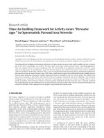
Inordertotesttheeffectiveness of the proposed BISN
algorithm, recognition experiments were performed on two
different databases that address different adverse conditions.
We believe that it is important to test the speaker normal-
ization algorithms for actual adverse environments, in order
to determine if they have practical value. The databases used
in the simulations are (a) CU-Move database-extended digits
Portion [30], for real noisy in-car environments, (b) speech
in noisy environments (SPINEs) [31], for simulated noisy
military task conditions. These databases reflect good exam-
ples of environments where reliable and efficient speaker
normalization is needed.
6.1. General system description
For all experiments, we used SONIC [32, 33], the University
of Colorado’s HMM-based large vocabulary speech recogni-
tion system. We used a window length of 25 milliseconds and
a skip rate of 10 milliseconds by Hamming windowing the
frame data before further processing. The 39-dimensional
feature set contains 12 statics, deltas and delta-deltas along
with normalized-log energy, delta and delta-delta energy.
Cepstral mean normalization (CMN) was utilized on the
final feature vectors.

For both VTLN and BISN experiments, a single best warp
is estimated for each speaker offline using all available data.
We re-extracted PMVDR features using these best warps and
retrained the HMM model set in order to obtain canonical
models. During the test, a two-pass strategy was used. First,
all utterances from a single speaker are recognized with
Table 1: WERs[%] for CU-Move in-vehicle task with different front
ends/speaker normalization algorithms.
System/WER Female Male Overall
MFCC 9.16 13.22 11.12
PMVDR 5.57 8.76 7.11
PMVDR w/Spkr. norm.
VTLN 4.30 7.12 5.66
BISN 4.16 7.17 5.61
BISN w/BTS 4.16 7.17 5.61
BISN w/MS-BTS 4.13 7.16 5.59
noncanonical HMM set, and best warp factors are estimated
using the result of this recognition. In the second step, the
utterances for that speaker are extracted incorporating the
best warps obtained in the first step, and a second recognition
is performed with the canonical models to get the final
hypothesis.
6.2. Experiments for CU-Move extended digits task
For noisy speech experiments, we use the CU-Move extended
digits corpus [30] which was collected in real car environ-
ments. The database and noise conditions are analyzed in
[34, 35]indetail.
A total of 60 speakers balanced across gender and age
(18–70 years old) were used in the training set. (Note that
[34] summarizes recommended training development and

test sets for the CU-Move corpus.) The test set contained
another 50 speakers, again gender and age balanced. The
HMMs were trained using SONIC’s decision-tree HMM
trainer [32, 33] resulting in a model set with approxi-
mately 10 K total Gaussians. The 40-word vocabulary is
very convenient for telephone dialing applications since it
contains many necessary words like “dash”, “pound”, “sign”
in addition to numbers. We used the optimized settings (α
=
0.57 and P = 24) for PMVDR on the CU-Move task [3].
The recognition performance for different normalization
approaches is given in Ta b le 1 . As we can see, the relative
improvement of PMVDR integrated with BISN is close to
50% WER reduction with respect to the MFCC baseline.
Although there is no substantial improvement in the
WER performance of the BISN-based techniques with
respect to VTLN baseline, there is a computational gain and
the convenience of performing the recognition within the
acoustic front end merely changing an internal parameter.
BISN-based normalization can be easily integrated into
embedded systems, such as in-car speech-based navigation
systems, without increasing the computational cost signifi-
cantly.
6.3. Experiments for the SPINE task
The SPINE task uses the ARCON communicability exercise
(ACE) that was originally developed to test communication
systems. The training data for the SPINE-2 task consists of
4 parts, (1) SPINE-1 training data (8.7 hours), (2) SPINE-
1 evaluation data (7.3 hours), (3) SPINE-2 training data
U. H. Yapanel and J. H. L. Hansen 9

Table 2: WERs[%] for SPINE task with different front ends/speaker
normalization algorithms.
System/WER Female Male Overall
MFCC 43.91 39.70 41.81
PMVDR 43.14 39.57 41.36
VTLN 39.62 36.92 38.28
BISN 39.56 36.94 38.25
BISN w/BTS 39.56 36.94 38.25
BISN w/MS-BTS 39.75 36.76 38.26
(3.4 hours), and (4) SPINE-2 development data (1.1 hours)
totaling up to 20.5 hours of training data. The evaluation
data consists of 64 talker-pair conversations which is 3.5
hours of total stereo data (2.8 hours of talk-time total).
On the average, each of the 128 conversations contains 1.3
minutes of speech activity. For the SPINE-2 evaluation, a
class N-gram language model is trained from the training
data text. For further details about the task, we refer readers
to [33]. The test data contains large segments of silence and
a voice activity detector (VAD) is used to estimate speech
segments. For the speaker normalization experiments, how-
ever, we preferred to use reference hand-cuts provided by
NRL in order to objectively evaluate the performance of
speaker normalization algorithms. We again trained gender-
independent HMMs using the Sonic’s decision-tree HMM
trainer. The models had about 2500 clusters and around
50 K Gaussians. We used α
= 0.42 (Mel scale at 16 kHz)
and P
= 24 as the settings for the PMVDR front end. The
recognition performance for different speaker normalization

approaches is given in Tabl e 2 . The relative improvement of
PMVDR w/BISN is about 8.5% WER reduction with respect
to the MFCC baseline. This moderate improvement can be
attributed to the high WER of the task. Since the recognition
results (hence the alignments) are not sufficiently accurate,
this yields poor warp estimates. Again the WER performance
is comparable with VTLN. We observe a better improvement
for females versus males from the MFCC baseline.
7. APPLICATION OF BISN IN A REAL-TIME SCENARIO
We now would like to elaborate on the application of BISN
w/MS-BTS within a real world scenario. In real time, we
have all the training data in advance and can determine the
self-normalization warps offline using all the available data
from each speaker. However, during the test we do not have
access to all speech from a specific speaker to determine
the self-normalization warp for that speaker. Moreover, we
do not have the information as to when speaker changes
occur. So the algorithm should in fact be able to adapt the
self-normalization warps to changing speakers. It should
also be flexible (i.e., slowly changing) even for the same
speaker to account for the slight variations in the vocal-tract
characteristics. By making effective use of all the algorithms
described so far, it is possible to establish a cooperation
between the acoustic front end and the recognizer which will
enable the front end to normalize itself automatically without
the need to perform recognition twice. We give the block-
diagram for the application of this self-normalization front
end (BISN w/MS-BTS) in Figure 4.
Assume that we have the canonical models, λ
N

, trained
on speaker-normalized training data and would like to
perform online VTLN during the test. Also assume that
recognition is performed for small sections of speech (i.e.,
utterances). We can summarize the operation of the self-
normalizing front end as follows.
(i) Parameterize first the nth input utterance with the
perceptual warp α
avg
(n).
(ii) Recognize the utterance and pass the transcription
(with alignment) information A
n
to the MS-BTS
block.
(iii) Determine the best self-normalization warp (i.e., the
instantaneous warp α
ins
(n) for the current utterance
n).
(iv) Pass α
ins
(n) through a recursive averaging block with
a forgetting factor(β)toobtainanaveragedversion
(i.e., α
avg
(n + 1)). Here, the forgetting factor β was
set to 0.6, an optimization experiment is presented in
this chapter later on.
(v) Supply α

avg
(n + 1) to the PMVDR front end, which
is an estimate of the self-normalization warp for the
n +1thincoming utterance.
In summary, the front end estimates the self-normalization
warp for the incoming utterance by using the self-
normalization warp estimated from the earlier utterances via
a recursive averaging with a forgetting factor. After perform-
ing recognition with the estimated self-normalization warp,
the recognizer feeds back the alignment information so that
the self-normalization warp for the next utterance can be
estimated (and updated).
In this way, we never have to perform the recognition
twice and sequentially we refine the warp estimate to
accommodate the slight variations for the vocal-tract even
for the same speaker. Moreover, the recursive averaging
ensures quick adaptation of self-normalization warp to
changing speakers over time. If we call the instantaneous warp
estimated for the current utterance α
ins
(n), then the self-
normalization warp estimate for the incoming utterance can
be computed as follows:
α
avg
(n +1)= α
ins
(n)(1 −β)+α
avg
(n)β, n = 0, 1, , N,

(17)
where α
avg
(n) is the averaged warp used in the parameter-
ization of nth utterance, α
ins
(n) is the instantaneous warp
estimated for the nth utterance given the features from
the front end X
n
and alignment from the recognizer A
n
,
and α
avg
(n + 1) is the estimated warp factor to be used in
the parameterization of (n + 1)th utterance. As an initial
condition for the first utterance, we can choose to use the
center warp of our search space (i.e., α
avg
(0) = α
C
= 0.57).
Finally, N is the total number of utterances in the test set. β
provides a means for smoothing the self-normalization warp
estimate and helps accounting for the changes in vocal-tract
characteristics. Since the instantaneous self-normalization
10 EURASIP Journal on Audio, Speech, and Music Processing
1G HMM set
Optimal warp search

via model-based binary
tree search (MS-BTS)
Aligned utterance (An)
α
ins
(n)
Recursive averaging
with
forgetting factor, β
α
avg
(n +1)
Recognizer
&
aligner
nth input utterance
PMVDR
acoustic front-end
(α
avg
(n), P)
Features (Xn)
Self-normalizing front-end (PMVDR w/BISN)
Output (Wn)
Canonical HMMs
Figure 4: The block diagram of the self normalizing front end (PMVDR w/BISN) in a real-word application scenario.
Table 3: WERs[%] for CU-Move task with offline and on-the-fly
BISN.
System/WER Female Male Overall
PMVDR 5.57 8.76 7.11

BISN w/MS-BTS (off-line) 4.13 7.16 5.59
BISN w/MS-BTS (on-the-fly) 3.90 7.04 5.42
warp α
ins
(n) is estimated from a short segment of data
(as short as one spoken digit), it fluctuates considerably.
We give the variation of instantaneous self-normalization
warp (α
ins
(n)) and recursively averaged self-normalization
warp (α
avg
(n)) for a comparison in Figure 5. The fixed self-
normalization warps obtained from the offline BISN w/MS-
BTS algorithm are also superimposed on the averaged self-
normalization warp graph. The averaged self-normalization
warp tracks the fixed self-normalization warp, permitting
slow variations within the same speaker. Allowing some
flexibility for the warp factor even within the same speaker
compensates for variations which may stem from Lombard
effect, stress, or a number of other physiological factors [36].
It is also shown that the averaged self-normalization warp
successfully and quickly adapts to new speakers with no need
to detect speaker turns.
As observed from Figure 5, the fluctuation in instan-
taneous self-normalization warp is mostly smoothed out
by the recursive averaging. To determine a good value for
the forgetting factor β,weconductedanexperimentfora
changing forgetting factor β versus WER, the results are
presented in Figure 6. As observed, the particular value of β

is not that crucial as long as it is within the range of [0.4–
0.8]. We infer that, for the CU-Move task, a good value of the
forgetting factor (β)is0.6.
In Ta bl e 3, we summarize the recognition results for
the CU-Move task in which each test speaker had an
average of approximately 60 utterances. The results, which
0.5
0.55
0.6
0.65
0.7
Self-normalization warp
0 50 100 150 200 250 300 350
Number of utterances (n)
Fixed
SNW
Averaged SNW
Instantenous
SNW
Figure 5: The variation of the instantaneous self-normalization
warp (α
i
(n)), averaged self-normalization warp (α
a
(n)), and fixed
self-normalization warp (obtained from offline BISN w/MS-BTS),
the speaker turns are also marked with a dashed line (the averaged
self-normalization warp and fixed self-normalization warp are
shifted upwards by 0.1 for proper illustration).
are slightly better than the offline experimentation, confirm

the applicability of the proposed self-normalizing front
end (BISN w/MS-BTS). This can be attributed to the
more accurate alignments obtained during the on-the-fly
normalization. In the offline case, all speech for a specific
speaker is recognized first and then a warp factor is
determined, since unwarped models and features are used
in the first round of recognition, the recognition results
(hence alignments) are moderately accurate. In the on-the-
fly experimentation, however, the warp is adjusted as more
and more data becomes available from the same speaker, and
normalized models and features are used to update the self-
normalization warp, hence the alignments supplied by the
U. H. Yapanel and J. H. L. Hansen 11
5.4
5.6
5.8
6
6.2
6.4
6.6
6.8
7
Word e r ro r r ate ( W ER)
0.30.40.50.60.70.80.9
Forgetting factor
Figure 6: The variation of the WER with the forgetting factor (β).
recognizer are more accurate, yielding better estimates for
the self-normalization warp. We also note that for Ta bl e 3 ,
it is not possible to directly compare BISN w/MS-BTS with
VTLN, since VTLN can only be applied offline.

8. COMPUTATIONAL CONSIDERATIONS
This final section aims to evaluate all algorithms in terms
of their computational efficiency. We consider the number of
warpings performed on the FFT spectrum (NW), the number
of feature extractions (NFEs) required for the whole system
(both for search and recognition), the number of likelihood
computations (NLCs), and lastly the number of recognition
passes (NRPs). Ta ble 4 clearly illustrates the computational
gain obtained by moving from classical VTLN to the on-the-
fly version of BISN w/MS-BTS. Moving from classical VTLN
to BISN eliminates the need to perform warping on the FFT
spectrum twice. The perceptual and speaker normalization
warps are integrated into a single speaker-dependent warp.
Integration of the MS-BTS algorithm within the BISN
framework for an on-the-fly application eliminates even the
need to extract the features twice. Extracted features for
recognition are also passed to the MS-BTS block for the self-
normalization warp estimation for the incoming utterance.
Since the estimation is sequential, the need to perform
recognition twice is also eliminated. The self-normalization
warp for the incoming utterance is recursively estimated
from earlier utterances. The computational load is now
reduced to realistic levels even for embedded systems. The
only drawback is that we need to store all single-Gaussian
models trained at each point of the search space (here we
have 17 single-Gaussian models in the BISN case) in memory
all the time. However, since these are only single-Gaussian
models, they do not require a large amount of memory.
9. CONCLUSIONS
In this paper, we have proposed a new and efficient algorithm

for performing online and efficient VTLN which can easily
Table 4: Computational complexity for different speaker normal-
ization algorithms. (NWs: number of warpings, NFEs: number
of feature extractions, NLCs: number of likelihood computations,
NRPs: number of recognition passes).
Algorithm NW
NFE
NLC NRP
(Search + Recog.)
VTLN 2 18 + 1 18 2
BISN 1 10 + 1 10 2
BISN w/BTS 1 6 + 1 6 2
BISN w/MS-BTS (off-line) 1 1 + 1 6 2
BISN w/MS-BTS (on-the-fly) 1 0 + 1 6 1
Total gain [%] 50.094.766.750.0
be implemented within the PMVDR front end. In VTLN,
we need to perform warping on the spectrum twice,to
accommodate perceptual considerations and to normalize
for speaker differences. The proposed BISN algorithm, on
the other hand, estimates a self-normalization warp for
each speaker which performs both the perceptual warp and
speaker normalization in a single warp. The use of a single
warp to achieve both perceptual warp and VTLN warp
unifies these two concepts. The model space-binary tree
search (MS-BTS) algorithm was integrated to reduce the
computational load in the search stage for the estimation
of self-normalization warps. Moving the search base from
the feature space to the model space [13] reduced the need
to extract the features for each point in the search space,
which in turn eliminated the need for high computational

resources. A sequential on-the-fly implementation of the
BISN w/MS-BTS algorithm also eliminated the need to
perform multipass recognition which makes it possible to
integrate this scheme with low-resource speech recognition
systems.
We have shown that the BISN approach is effective
for two different databases, the CU-Move in-vehicle dialog
(extended digits portion) database and the SPINE military
noisy speech database. The on-the-fly implementation of the
BISN w/MS-BTS algorithm was also shown to be slightly
more accurate than the offline version with a considerable
savings in computational resources. Integrated with the BISN
approach, the PMVDR front end can now be considered an
intelligent front end which cooperates with the recognizer
in order to automatically normalize itself with respect to
the incoming speaker/speech. Since it can quickly adapt to
the changing vocal-tract characteristics, it does not require
any detection of speaker changes whatsoever. We believe
that the PMVDR front end integrated with the strong
BISN algorithm is an ideal front end for use in every
system requiring noise robustness and a measurable level
of speaker normalization (especially for embedded systems).
It can perform acoustic feature extraction with moderate
computational requirements and achieve self-normalization
with respect to changing speakers very efficiently, yielding
a sound acoustic front end that can be used in today’s
demanding speech recognition applications.
12 EURASIP Journal on Audio, Speech, and Music Processing
SUMMARY OF ABBREVIATIONS AND ACRONYMS
1G: Single-Gaussian

ACE: Arcon communicability exercise
APT: All-pass transform
ASR: Automatic speech recognition
BISN: Built-in speaker normalization
BTS: Binary tree search
BLT: Bilinear transform
CDHMM: Continuous density hidden Markov model
CMN: Cepstral mean normalization
DRT: Diagnostic rhyme test
FFT: Fast Fourier transform
GMM: Gaussian mixture model
HMM: Hidden Markov model
IFFT: Inverse fast Fourier transform
LDA: Linear discriminant analysis
LP: Linear prediction
LPC: Linear predictive coding
LPCCs: Linear prediction-based cepstral coefficients
MFCCs: Mel-frequency cepstral coefficients
MS-BTS: Model space binary tree search
MVDR: Minimum variance distortionless response
NFE: Number of feature extraction
NLC: Number of likelihood computation
NRPs: Number of recognition passes
NWs: Number of warps
PMVDR: Perceptual MVDR cepstral coefficients
SNW: Self-normalization warp
SPINEs: Speech in noise evaluations
TM: Trace measure
VAD: Voice activity detector
VTLN: Vocal-tract length normalization

VTTF: Vocal-tract transfer function
WER: Word error rate.
ACKNOWLEDGMENT
This work was supported by US Air Force Research Labora-
tory, Rome NY, under Contract no.FA8750-04-1-0058.
REFERENCES
[1] M. J. Hunt, “Spectral signal processing for ASR,” in Proceedings
of the IEEE Workshop on Automatic Speech Recognition and
Understanding (ASRU ’99), vol. 1, pp. 17–26, Keystone, Colo,
USA, December 1999.
[2]U.H.YapanelandJ.H.L.Hansen,“Anewperspectiveon
feature extraction for robust in-vehicle speech recognition,”
in Proceedings of the 8th European Conference on Speech
Communication and Technology (EUROSPEECH ’03),pp.
1281–1284, Geneva, Switzerland, September 2003.
[3]U.H.YapanelandJ.H.L.Hansen,“Anewperceptually
motivated MVDR-based acoustic front-end (PMVDR) for
robust automatic speech recognition,” Speech Communication,
vol. 50, no. 2, pp. 142–152, 2008.
[4] J. H. L. Hansen, “Analysis and compensation of speech under
stress and noise for environmental robustness in speech
recognition,” Speech Communication, vol. 20, no. 1-2, pp. 151–
173, 1996.
[5] J. H. L. Hansen, “Morphological constrained feature enhance-
ment with adaptive cepstral compensation (MCE-ACC) for
speech recognition in noise and Lombard effect,” IEEE
Transactions on Speech and Audio Processing,vol.2,no.4,pp.
598–614, 1994.
[6] L. Lee and R. C. Rose, “Speaker normalization using efficient
frequency warping procedures,” in Proceedings of the IEEE

International Conference on Acoustics, Speech, and Signal
Processing (ICASSP ’96), vol. 1, pp. 353–356, Atlanta, Ga, USA,
May 1996.
[7] L. Lee and R. C. Rose, “A frequency warping approach
to speaker normalization,” IEEE Transactions on Speech and
Audio Processing, vol. 6, no. 1, pp. 49–60, 1998.
[8] A. Andreou, T. Kamm, and J. Cohen, “Experiments in vocal
tract normalization,” in Proceedings of the CAIP Workshop:
Frontiers in Speech Recognition II,Piscataway,NJ,USA,July-
August 1994.
[9] E. Eide and H. Gish, “A parametric approach to vocal tract
length normalization,” in Proceedings of the IEEE International
Conference on Acoustics, Speech, and Signal Processing (ICASSP
’96), vol. 1, pp. 346–348, Atlanta, Ga, USA, May 1996.
[10] A. Acero, Acoustical and environmental robustness in automatic
speech recognition, Ph.D. thesis, Carnegie Mellon University,
Pittsburgh, Pa, USA, 1990.
[11] J. McDonough, Speaker compensation with all-pass transforms,
Ph.D. thesis, The John Hopkins University, Baltimore, Md,
USA, 2000.
[12] J. McDonough, W. Byrne, and X. Luo, “Speaker adaptation
with all-pass transforms,” in Proceedings of the 5th Interna-
tional Conference on Spoken Language Processing (ICSLP ’98),
vol. 6, pp. 2307–2310, Sydney, Australia, November-December
1998.
[13] T. Hain, P. C. Woodland, T. R. Niesler, and E. W. D.
Whittaker, “The 1998 HTK system for transcription of
conversational telephone speech,” in Proceedings of the IEEE
International Conference on Acoustics, Speech, and Signal
Processing (ICASSP ’99), pp. 57–60, Phoenix, Ariz, USA,

March 1999.
[14] R. Sinha and S. Umesh, “A method for compensation of
Jacobian in speaker normalization,” in Proceedings of the
IEEE International Conference on Acoustics, Speech, and Signal
Processing (ICASSP ’03), vol. 1, pp. 560–563, Hong Kong, April
2003.
[15] R. Haeb-Umbach, “Investigations on inter-speaker variability
in the feature space,” in Proceedings of the IEEE Interna-
tional Conference on Acoustics, Speech, and Signal Processing
(ICASSP ’99), vol. 1, pp. 397–400, Phoenix, Ariz, USA, March
1999.
[16] Y. Kim, Signal modeling for robust speech recognition with
frequency warping and convex optimization, Ph.D. thesis,
Department of Electrical Engineering, Stanford Univerity,
Palo Alto, Calif, USA, May 2000.
[17]M.N.MurthiandB.D.Rao,“All-polemodelingofspeech
based on the minimum variance distortionless response
spectrum,” IEEE Transactions on Speech and Audio Processing,
vol. 8, no. 3, pp. 221–239, 2000.
[18] B. R. Musicus, “Fast MLM power spectrum estimation
from uniformly spaced correlations,” IEEE Transactions on
Acoustics, Speech, and Signal Processing,vol.33,no.5,pp.
1333–1335, 1985.
[19] J. O. Smith III and J. S. Abel, “Bark and ERB bilinear
transforms,” IEEE Transactions on Speech and Audio Processing,
vol. 7, no. 6, pp. 697–708, 1999.
U. H. Yapanel and J. H. L. Hansen 13
[20] K. Tokuda, T. Masuko, T. Kobayashi, and S. Imai, “Mel-
generalized cepstral analysis-a unified approach to speech
spectral estimation,” in Proceedings of the International Con-

ference on Spoken Language Processing (ICSLP ’94), pp. 1043–
1046, Yokohama, Japan, September 1994.
[21] S. Haykin, Adaptive Filter Theory, Prentice-Hall, Englewood
Cliffs, NJ, USA, 1991.
[22] J. Makhoul, “Linear prediction: a tutorial review,” Proceedings
of the IEEE, vol. 63, no. 4, pp. 561–580, 1975.
[23] A. V. Oppenheim and R. W. Schafer, Di screte-Time Signal
Processing, Prentice-Hall, Englewood Cliffs, NJ, USA, 1989.
[24] U. H. Yapanel, Acoustic modeling and speaker normalization
strateg ies with application to robust in-vehicle speech recognition
and dialect classification, Ph.D. thesis, Robust Speech Process-
ing Group - CSLR, Department of Electrical and Computer
Engineering, Univerity of Colorado at Boulder, Boulder, Colo,
USA, 2005.
[25] U. H. Yapanel, S. Dharanipragada, and J. H. L. Hansen,
“Perceptual MVDR-based cepstral coefficients (PMCCs) for
high accuracy speech recognition,” in Proceedings of the 8th
European Conference on Speech Communication and Technol-
og y (EUROSPEECH ’03), pp. 1829–1832, Geneva, Switzerland,
September 2003.
[26] J. H. L. Hansen, X. Zhang, M. Akbacak, et al., “CU-MOVE:
advanced in-vehicle speech systems for route navigation,” in
DSP for In-Vehicle and Mobile Systems, chapter 2, pp. 19–45,
Springer, New York, NY, USA, 2005.
[27] P. Zhan and M. Westphal, “Speaker normalization based
on frequency warping,” in Proceedings of the IEEE Interna-
tional Conference on Acoustics, Speech, and Signal Processing
(ICASSP ’97), vol. 2, pp. 1039–1042, Atlanta, Ga, USA, April
1997.
[28] LDC, />catalogId

=LDC93S6A.
[29] M. Pitz, S. Molau, R. Schluter, and H. Ney, “Vocal tract
normalization equals linear transformation in cepstral space,”
in Proceedings of the 7th European Conference on Speech Com-
munication and Technology (EUROSPEECH ’01),Aalborg,
Denmark, September 2001.
[30] CSLRCU-Move corpus, now maintained at, http://www
.utdallas.edu/research/utdrive/.
[31] J. H. L. Hansen, R. Sarikaya, U. H. Yapanel, and B. Pel-
lom, “Robust speech recognition in noise: an evaluation
using the SPINE corpus,” in Proceedings of the 7th Euro-
pean Conference on Speech Communication and Technology
(EUROSPEECH ’01) , vol. 2, pp. 905–908, Aalborg, Denmark,
September 2001.
[32] B. Pellom, “SONIC: the university of colorado continuous
speech recognizer,” Tech. Rep. TR-CSLR-2001-01, Center for
Spoken Language Research, University of Colorado at Boulder,
Boulder, Colo, USA, March 2001.
[33] B. Pellom and K. Hacioglu, “Recent improvements in the
CU Sonic ASR system for noisy speech: the SPINE task,” in
Proceedings of the IEEE International Conference on Acoustics,
Speech, and Signal Processing (ICASSP ’03), vol. 1, pp. 4–7,
Hong Kong, April 2003.
[34] J. H. L. Hansen, “Getting started with CU-Move database,”
Tech. Rep., Robust Speech Processing Group - CSLR,
Boulder, Colo, USA, March 2002, />research/utdrive/.
[35] J. H. L. Hansen, P. Angkititrakul, J. Plucienkowski, et al.,
“CU-move: analysis & corpus development for interactive
in-vehicle speech systems,” in Proceedings of the 7th Euro-
pean Conference on Speech Communication and Technol-

og y (EUROSPEECH ’01), pp. 209–212, Aalborg, Denmark,
September 2001.
[36] S. E. Bou-Ghazale and J. H. L. Hansen, “A comparative study
of traditional and newly proposed features for recognition of
speech under stress,” IEEE Transactions on Speech and Audio
Processing, vol. 8, no. 4, pp. 429–442, 2000.