Hindawi Publishing Corporation
EURASIP Journal on Wireless Communications and Networking
Volume 2009, Article ID 721301, 12 pages
doi:10.1155/2009/721301
Research Article
An Empirical Model for Probability of Packet Reception in
Vehicular Ad Hoc Networks
Moritz Killat and Hannes Hartenstein
Institute of Telematics, University of Karlsruhe, Zirkel 2, 76131 Karlsruhe, Germany
Correspondence should be addressed to Moritz Killat,
Received 3 May 2008; Revised 7 September 2008; Accepted 28 November 2008
Recommended by Onur Altintas
Today’s advanced simulators facilitate thorough studies on VANETs but are hampered by the computational effort required to
consider all of the important influencing factors. In particular, large-scale simulations involving thousands of communicating
vehicles cannot be served in reasonable simulation times with typical network simulation frameworks. A solution to this
challenge might be found in hybrid simulations that encapsulate parts of a discrete-event simulation in an analytical model while
maintaining the simulation’s credibility. In this paper, we introduce a hybrid simulation model that analytically represents the
probability of packet reception in an IEEE 802.11p network based on four inputs: the distance between sender and receiver,
transmission power, transmission rate, and vehicular traffic density. We also describe the process of building our model which
utilizes a large set of simulation traces and is based on general linear least squares approximation techniques. The model is
then validated via the comparison of simulation results with the model output. In addition, we present a transmission power
control problem in order to show the model’s suitability for solving parameter optimization problems, which are of fundamental
importance to VANETs.
Copyright © 2009 M. Killat and H. Hartenstein. This is an open access article distributed under the Creative Commons
Attribution License, which permits unrestricted use, distribution, and reproduction in any medium, provided the original work is
properly cited.
1. Introduction
The forecasted rise in transport demand poses a huge
challenge for intelligent transportation systems (ITSs). In
Europe alone, road transport will have increased by 50%
between 1990 and 2010 [1]. The increase in trafficwillnot

only impact the road network itself, 10% of which is expected
to experience jams once per day across the continent by 2010,
but also traffic safety and the environment.
The application of emerging technologies like vehicular
ad hoc networks (VANETs) might help to mitigate some of
the adverse effects related to the rising demand. Presumably,
the direct wireless exchange of information between vehi-
cles will enable drivers to communicate and thus lead to
improvements in trafficefficiency and safety. This technology
will also enable vehicles to better exploit the capacity of
the road network and to alert each other to oncoming
dangers. However, as intuitive as the potential benefits may
be, the implementation of the new technologies will require
immense sophistication because wireless communication in
a vehicular environment is subject to challenging radio
conditions. The multitude of communicating nodes all
accessing the limited communication channel and the high
mobility of radio-signal-reflecting objects complicate the
successful transmission of data.
With respect to the communication challenges that arise
in VANETs, one-hop broadcast communication is a key com-
ponent of inter-vehicle communication. In this paper, we will
elaborate upon this key primitive and present an analytical
model that gives the probability of successfully receiving a
one-hop broadcast message based on the distance between
sender and receiver, transmission power, transmission rate,
and vehicular traffic density. The applicability of this model
is at least twofold.
(1) Hybrid simulations. Nowadays, computer simulations
are the primary means of studying the efficacy of

VANETs. Although very advanced simulators are
2 EURASIP Journal on Wireless Communications and Networking
currently available, the computational effort required
to obtain credible simulation results limits the sim-
ulators’ applicability, especially, for large-scale simu-
lations involving thousands of communicating vehi-
cles. By the 1970s, researchers were already proposing
the use of hybrid simulations that combined math-
ematical modeling with discrete-event simulations;
see, for example, [2]. This hybrid approach was
able to reduce computation time by some orders of
magnitude. Regarding simulations in VANETs, for
instance, [3] have shown in a sample scenario that a
hybrid approach accelerates the simulation study by
a factor of 500. The basic building block of a hybrid
approach, however, is a suitable model that maintains
the accuracy of a pure discrete simulation.
(2) Solving optimization problems. On the road, vehicles
need to autonomously choose the communication
parameters that best fit an application’s needs. The
complexity of the numerous influencing factors,
however, impedes the determination of an appro-
priate configuration. One could instead formulate
and solve a corresponding optimization problem to
achieve the same purpose; however, an appropriate
model of the communication behavior is required.
In this paper, we address the development of just such a
model. In detail, our contributions are as follows.
(1) Model building. From a large set of simulation traces
we derive an empirical model that provides the prob-

ability of one-hop broadcast reception in an IEEE
802.11p network. The application of curve fitting
techniques provides an analytical expression for the
probability of packet reception that allows accurate
interpolation between simulated data points. Our
model holds for varying conditions in four dimen-
sions: (i) distance between sender and receiver, (ii)
transmission rate, (iii) transmission power, and (iv)
vehicular traffic density.
(2) Model validation. We demonstrate the validity of
the model by addressing the issue of optimal trans-
mission power assignment from two perspectives:
numerically gained solutions of optimization prob-
lems versus results of computer simulations.
The remaining part of this paper is structured as follows:
in Section 2 we take a look at the literature and summarize
previous papers on topics related to modeling issues in
wireless communication systems. Section 3 deals with the
model building process. We delineate our key assumptions
and comprehensively describe our methodological approach,
which employs analytical derivation and general linear least
squares curve fitting. Section 4 addresses the validation of
the derived model by statistical and application means.
We consider the problem of optimal transmission power
assignment and compare simulative results with numerically
computed solutions. Finally, we conclude the paper in
Section 5.
2. Related Work
To the best of our knowledge, no analytical model on
communication characteristics has been published that

considers all of the particularities of a vehicular environment.
Wireless local area networks in general, however, have
been exemplarily studied by Bianchi, who modeled the
IEEE 802.11 standard by means of Markov Chains [4].
Although his analysis is restricted to certain assumptions,
Bianchi has shown strong conformance between the model
and simulative results. Bianchi’s paper has spawned many
follow-up papers that relax his assumptions, correct flaws,
and propose extensions to his model. In [5], for instance,
the authors corrected Bianchi’s IEEE 802.11 modeling by
allowing for packet drops caused by contention by revising
the assumption of (potentially) infinite retransmissions by a
node. The work in [6–8] incorporated a nonidealistic sensing
of the radio channel and thus addressed the problem of
hidden terminals. The work in [9, 10] digressed from the
assumption of saturated conditions on the communication
channel and [11] additionally introduced a probabilistic
radio wave propagation. A deep mathematical analysis was
proposed in [12] that studies a probabilistic radio wave
propagation and the capturing effect. The complexity of a
joint consideration of all effects, however, has thwarted the
proposition of a complete model that reflects IEEE 802.11
communication behavior.
In [3] Killat et al. discussed empirical model building for
the simulation of vehicular ad hoc networks. By exploiting
simulation traces of an advanced communication simulator,
the authors derived an empirical model that mirrored the
communication behavior of the corresponding discrete-
event simulations. Their model’s limitation to tight scenario
configurations is addressed and compensated for in the

present paper.
A fundamental contribution to modeling in wireless
communication networks has been made by Jiang et al. [13].
They defined the communication density as the product of
transmission rate, transmission power, and trafficdensity
and have shown that equal communication densities evince
very similar communication characteristics. We will make
use of this relationship in our model-building process.
Finally, we refer to advanced communication simula-
tors for vehicular ad hoc networks that have thoroughly
considered impacts on wireless communication systems.
Employing the widely used network simulator ns-2 [14],
Chen et al. provided emendations to address the effects that
are especially relevant in a vehicular environment [15]. Their
work has enabled researchers to improve existing analytical
models. Chen et al.’s simulator will serve as the basis for the
empirical model presented in the following.
3. Model Building
This section addresses the construction of an empirical
model that represents the probability of successfully receiv-
ing one-hop packet transmissions under various circum-
stances. The model is conceived as a flexible tool for
developers to use in the application design process and thus
EURASIP Journal on Wireless Communications and Networking 3
takes varying traffic conditions into account. Therefore, we
span the problem space as follows: assuming a trafficdensity
of δ vehicles per kilometer that all periodically broadcast
messages with a certain transmission power ψ at a rate f
and denoting the distance to the sender by x, the model M
provides the corresponding probability of one-hop packet

reception P
R
(x, δ, ψ, f ). While the distance as input factor
can naturally be explained by an attenuated radio signal over
distance, we consider the remaining three input dimensions
for the following reason. First of all, because all vehicles
communicate over a shared medium, communicating nodes
in close proximity need to cooperatively agree on adequately
time-separated transmissions if packet collisions are to
be avoided. As the number of neighboring nodes and
quantity of packets to be served increase, the coordination of
transmissions becomes more stressed. Hence, the frequency
of transmissions (and thus the amount of packets) and
the product of traffic density and communication distance
(and thus the number of nodes) become major indica-
tors for the challenge of collision-free distributed channel
allocation.
Clearly, the presented four input dimensions do not
completely cover the entire parameter space of the problem
at hand. Hence, we begin the following section by presenting
our key assumptions and delineate the model generation
process, which involves analytical and simulative derivations
and general linear least squares curve fitting techniques.
3.1. Assumptions. Our model assumes all nodes in the
network to communicate according to the IEEE 802.11p
draft standard [16], which offers a range of data transmission
rates from 3 Mbit/s to 27 Mbit/s. In [17] Maurer et al. argued
that lower data rates facilitate a robust message exchange
by offering better opportunities for countering noise and
interferences. In consideration of safety applications, which

are especially dependent on robust communication, we chose
the lowest data rate of 3 Mbit/s. The minimum contention
window of the IEEE 802.11 mechanisms was set to the
standard size of 15.
Regarding packet sizes, we assume all vehicles in the
scenario to transmit datagrams of equal size. Bearing in mind
that data packets require security protection, we allocate
128bytesforacertificate,54bytesforasignature,and
200 bytes of available payload, which adds up to a default
packet size of 382 bytes.
A key decision in VANET research concerns the assumed
radio wave propagation model. Early, simplistic proposals
assumed a deterministic attenuation of the radio signal
power over the transmission distance. However, as a suc-
cessful packet reception is determined by the comparison of
the received signal power to the noise level on the medium,
a deterministic reception behavior is thereby induced.
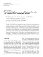
Figure 1 illustrates the deterministic characteristic in a
scenario containing a single sender only; we do not consider
interferences from simultaneous transmissions. Obviously,
a packet is received with certainty within the configured
communication range (here: 250 m). At any distance beyond
the communication range, however, message receptions
0
0.2
0.4
0.6
0.8
1
Probability of reception

0 100 200 300 400 500 600
Distance sender/receiver (m)
Deterministic propagation
Nakagami m
= 3
Figure 1: Probability of reception based on the distance between
sender and receiver. Comparison of deterministic and probabilistic
radio wave propagation models.
are ruled out. Clearly, this model hardly corresponds to
behavior we would expect in reality. Indeed, measurements
of inter-vehicle communications have shown a probabilistic
character. Due to the highly mobile environment and to
the multitude of reflecting objects, radio strengths vary at
certain distances over time. Taliwal et al. have shown that
the Nakagami-m distribution seems to suitably describe the
radio wave propagation in vehicular networks on highways
in the absence of interferences [18]. From the Nakagami
distribution we can consequently infer a probabilistic recep-
tion behavior, depicted also in Figure 1.Apparently,in
contrast to deterministic propagation models, we can no
longer identify a “communication range”. Nevertheless, a
deterministic model will henceforth be assumed whenever
we declare the transmission power for the Nakagami model,
that is, the power necessary to reach a communication range
of ψ meters. Additionally, in the following our study assumes
moderate radio conditions, expressed in a relaxed fast-
fading parameter (m
= 3) of the Nakagami-m distribution.
Varying channel conditions, that is, changing values of the
m-parameters, were not considered in the model-building

process.
Ta bl e 1 provides a detailed overview of the assumptions
applicable to the following simulation study.
3.2. Model Generation. A successful wireless packet reception
is determined by a number of influencing factors, such
as radio wave propagation and interferences issuing from
simultaneous transmissions. However, if only a single sender
is considered, the effects reduce to the specifics of the
environment and thus to the radio propagation. Under
this assumption, it was shown in [3] that the probability
of message reception can be analytically derived from the
4 EURASIP Journal on Wireless Communications and Networking
Table 1: Simulation configuration parameters.
Parameter Value
IEEE 802.11p data rate 3 Mbps
Frequency 5.9 GHz
Packet size 382 bytes
Antenna height 1.5 m
Antenna gain 4 dB
Minimum contention window 15 slots
Radio propagation model Nakagami m
= 3
Carrier sense threshold
−96 dBm
Noise floor
−99 dBm
SINR for preamble capture 4 dB
SINR for frame body capture 10 dB
Slot time 13 μs
SIFS time 32 μs

Preamble length 32 μs
PLCP header length 13 μs
Nakagami m = 3 model (for completeness, the derivations
are given in the appendix) as follows:
P
R
(x, δ, ψ, f ) = P
single
R
(x, ψ)
= e
−3(x/ψ)
2

1+3

x
ψ

2
+
9
2

x
ψ

4

.

(1)
In the most plausible scenario of many senders, the prob-
ability of reception is based on a plurality of factors.
For example, IEEE 802.11p MAC contentions, the hidden
terminal problem, and the capturing effect all effect message
reception but are very difficult to express analytically. For
this reason, we decided to pursue a hybrid approach: by
applying linear least squares curve fitting techniques to an
abundance of simulation traces, we obtain an analytical
term for the probability of reception. Additionally, we reveal
that dependencies exist between the varying input variables,
which will allow us to infer nonsimulated parameter setting
later on.
All of the simulations were conducted according to the
following scenario setup. In order to mimic varying highway
conditions, we pseudo-uniformly placed nodes on a straight
line to reflect the simulated trafficdensityδ.Inorderto
circumvent the “border effects” at the two ends of the road,
we based distance calculations on the arc length of a circle.
This approach essentially “eliminates” the two ends of the
road by creating a torus. All of the nodes broadcast packets at
the configured rate f with an equivalent transmission power
of ψ meters (cf. Section 3.1).
In each simulation, the receptions of packets sent out by
one specific node were recorded. To avoid correlations of
subsequent transmissions triggered by the node of interest,
we applied a relaxed transmission interval of one second to
the selected node. With a scenario duration of 100 seconds
and 30 seeds for each scenario, we thus captured up to 6000
packet receptions at each distance in every scenario (note that

each distance exists on both sides of the sender). The number
of simulated scenarios derives from all combinations in the
three dimensions:
traffic density (veh/km), δ: 25, 50, 75, 100, 200, 300,
400, 500,
transmission power (m), ψ: 100, 200, 300, 400, 500,
transmission rate (Hz), f :1,2,4,5,6,8,10,
which do not exceed a communication density of 500 packet
transmissions per second. This limit is based on the work
of Jiang et al., who defined communication density as the
product of transmission power, transmission rate, and traffic
density [13], which correspond to the number of packets
per second. Assuming our default packet size of 382 bytes, a
communication density of 500 corresponds to approximately
1.5 Mbit/s, or, when considering the entire neighborhood of
a vehicle, to 3 Mbit/s. Hence, larger communication densities
would exceed the capacity of available bandwidth and thus
might cause irregularities that are not addressed by our
model.
All simulations were run on an overhauled ns-2 network
simulator that takes account of specifics especially relevant
for inter-vehicle communications [15]. The system was
modified to more accurately model physical conditions,
considering the latest technology and improving flaws in
existing simulation frameworks [19].
The results of the numerous simulation runs agree with
the intuitive expectation that slight changes in the scenario
setup lead to only minor deviations in the probability
of reception. In more detail, when a single configuration
parameter (transmission power, transmission rate, vehicular

density) varies little, then we expect no abrupt deviation in
the probability of one-hop broadcast packet reception. Math-
ematically speaking, we suppose the probability of recep-
tion to be partially differentiable on the three-dimensional
interval that agrees with aforementioned restrictions on
the configuration parameters (e.g., communication density
not larger than 500). Figure 2 backs this supposition and
exemplarily depicts how the probability of reception varies
when configuration parameters change.
In order to obtain an empirical model from the simu-
lation runs, we applied the technique of linear least squares
curve fitting to each scenario trace. As suggested in [3],
expression (1) serves as a starting point and is then extended
with linear and cubic terms; in addition, fitting parameters
a
1
through a
4
are introduced:

P
R
(x, ψ) = e
−3(x/ψ)
2

1+
4

i=1

a
i

x
ψ

i

. (2)
Following the curve fitting process, expression (2)proved
to be an almost perfect match to the simulation traces
for all (
≈190) simulated scenarios. As a result of the
curve fits, we obtained a set of data points consisting of
the determined fitting parameters a
1
through a
4
for all
scenarios. Hence, we translated the dependencies pertinent
to our objective (probability of reception) from the tuple
(transmission power, transmission rate, vehicular density) to
EURASIP Journal on Wireless Communications and Networking 5
0
0.2
0.4
0.6
0.8
1
Probability of packet reception

500
400
300
200
100
Transmission power
ψ (m)
400
300
200
100
Vehicular density
δ (veh/km)
(a) Probability of reception at a distance of 200 m. Transmission
rate fixed at f
= 2Hz
0.1
0.3
0.5
0.7
Probability of packet reception
10
9
8
7
6
5
4
3
2

1
Transmission rate f (Hz)
300
200
100
Vehicular density
δ (veh/km)
(b) Probability of reception at a distance of 75 m. Transmission
power fixed at ψ
= 100 m
Figure 2: Probability of packet reception according to various configuration parameters.
−0.8
−0.6
−0.4
−0.2
0
Parameter a
1
50
150
250
350
Vehicular density (veh/km)
500
400
300
200
100
Transmission power (m)
(a) Parameter a

1
,txratefixedat f = 2Hz
2
3
4
5
6
7
Parameter a
2
10
9
8
7
6
5
4
3
2
1
Transmission rate (Hz)
100
200
300
400
500
Transmission
power (m)
(b) Parameter a
2

, vehicular density fixed at δ = 100 veh/km
−12
−8
−4
0
4
Parameter a
3
50
150
250
350
Vehicular density (veh/km)
500
400
300
200
100
Transmission power (m)
(c) Parameter a
3
,txratefixedat f = 2Hz
−1
1
3
5
Parameter a
4
10
9

8
7
6
5
4
3
2
1
Transmission rate (Hz)
300
200
100
0
vehicular density (veh/km)
(d) Parameter a
4
,txpowerfixedatψ = 100 m
Figure 3: Fitting parameters a
1
through a
4
based on configuration parameters.
the quadruple (a
1
, a
2
, a
3
, a
4

) and obtained the closed-form
analytical expressions (2).
Now, knowing that the fitting parameters a
1
through a
4
only depend on the configuration parameters and assuming
the differentiability of the probability of reception in the
configuration parameters, we infer the differentiability of the
fitting parameters in the configuration parameters. Again,
this conclusion is supported by Figure 3, which illustrates
the fitting parameters according to varying configuration
parameters. At this point, our concern was to find a
functional dependency that would allow us to choose the
appropriate fitting parameters for a given scenario configura-
tion. The assumed differentiability of the fitting parameters
in the configuration parameters allowed us to apply Taylor
series expansions to approximate the sought functional
dependency by means of a polynomial. In mathematical
6 EURASIP Journal on Wireless Communications and Networking
Parameter a
4
−3
1
5
Parameter a
3
−12
−8
−4

0
Parameter a
2
2
3.5
5
6.5
Parameter a
1
−2
−1.5
−1
−0.5
0
0 100 200 300 400 500
Communication density (ξ)
(a) Curve fit of a polynomial (fourth degree) to fitting parameters a
1
through a
4
based on the communication density ξ. a
4
in particular
shows considerable deviations from the fitted curve
Parameter a
4
0.5
0.7
0.9
Parameter a

3
0.8
0.9
1
Parameter a
2
0.7
0.8
0.9
1
Parameter a
1
0.8
0.9
1
Coefficient of determination (R
2
)
123456789
Degree of fitting polynomial
Communication density
tx power
(Communication density, tx power)
(b) Accuracy of fitting polynomials with varying degree to the configu-
ration parameter a
1
through a
4
Figure 4: Approximating configuration parameters a
1

through a
4
.
terms, we considered polynomial functions h
i
, i = 1, ,4,
which provide the corresponding fitting parameter a
i
for any
configuration parameter tuple, that is,
h
i
(δ, ψ, f ) =

j,k,l≥0
h
(j,k,l)
i
δ
j
ψ
k
f
l
≈ a
i
, i = 1, ,4, (3)
where h
(j,k,l)
i

are the coefficients. We obtained h
i
by approx-
imating each a
i
as closely as desired using a polynomial of
appropriate degree N and a linear least squares approxi-
mation algorithm. However, due to the three-dimensional
polynomial, the number of the coefficients h
(j,k,l)
i
for each a
i
rapidly increases even for small N values because the number
of coefficients h
(j,k,l)
i
is given by

N
n
=0
(
3+n−1
3
−1
) = (1/6)(N +
1)(N +2)(N + 3). Hence, instead of achieving accuracy at
the expense of complexity, in the resulting empirical model,
we decided to reduce complexity by applying generalizations,

such as communication density.
Inspired by Jiang et al.’s insights [13] of similar commu-
nication behavior in comparable communication densities,
we downgraded the three-dimensional polynomial h
i
to a
one-dimensional polynomial depending only on the com-
munication density ξ
= δ · ψ · f . Figure 4(a) illustrates that
even a polynomial of the fourth degree can conveniently
be fitted to a
1
through a
3
,butdifficulties (in terms of
noisy behavior) obviously arise for the remaining parameter
a
4
. This observation is likewise reflected in Ta bl e 2,which
provides the correlation coefficients of various configuration
parameter combinations to the fitting parameters a
1
through
a
4
.Incontrasttoa
4
, a
1
through a

3
shows a strong correlation
to ξ. On the other hand, a
4
is considerably correlated to
the transmission power parameter ψ. Thus, we decided to
apply a two-dimensional polynomial h
i
on the adjusted
communication density, ξ, and the transmission power, ψ,
which we fit to the dataset using the Levenberg-Marquardt
(for the curve fitting process we utilized the open source
software Gnu Regression, Econometric, and Time-series
Library (GRETL) version 1.7.1.) algorithm:
a
i
≈ h
i
(ξ, ψ) =

j,k≥0
h
(j,k)
i
ξ
j
ψ
k
,
i

= 1, ,4, with ξ = δ · ψ · f.
(4)
Regarding the degree of the two-dimensional polynomial,
we analyzed the impact of an increasing degree on the
accuracy of fitting parameter a
1
through a
4
. Figure 4(b)
illustrates the coefficient of determination R
2
of the fitting
process for various degrees. For each parameter, Figure 4(b)
depicts the fitting of a one-dimensional polynomial on
the most correlated configuration parameter and of a two-
dimensional polynomial on the most correlated parameter
and the communication density. Based on Figure 4(b),we
have chosen a two-dimensional polynomial of fourth degree
for all fitting parameters in expression (4), that is, j + k
≤ 4.
We thus state the sought empirical model
M:

P
R
(x, δ, ψ, f ) = e
−3(x/ψ)
2

1+

4

i=1
h
i
(ξ, ψ)

x
ψ

i

(5)
and list the coefficients obtained from the polynomial func-
tions h
i
(cf. expression (4)) in Tab le 3 . Note that although
some values in Tab le 3 seem to be negligible, a sensitivity
analysis has shown that if a single of the h
(j,k)
i
parameter is
omitted, deviations in the probability of reception from 8%
to 100% can be observed.
Finally, Figure 5 shows that in scenarios which only
contain a single sender ( f
= δ = 1) the obtained fitting
function h
1
through h

4
suitably conforms to the analytical
EURASIP Journal on Wireless Communications and Networking 7
Table 2: Correlation of fitting parameters a
1
through a
4
and various configuration parameter combinations.
ψδ fψ·δψ· fδ· fξ
a
1
−0.2564 −0.3983 −0.4125 −0.4655 −0.4728 −0.7449 −0.9581
a
2
0.2772 0.4163 0.4095 0.4690 0.4491 0.7019 0.8255
a
3
−0.3635 −0.3896 −0.3860 −0.5098 −0.5022 −0.6937 −0.9179
a
4
0.7148 −0.0667 −0.0351 0.3493 0.4060 0.0364 0.4712
Table 3: Coefficients h
(j,k)
i
subjected to the polynomials h
1
through h
4
. Although some values seem to be negligible, all values significantly
influence the resulting probability of reception.

(j, k)
(0,0) (1,0) (2,0) (3,0) (4,0)
h
(j,k)
1
0.0209865 −9.66304e − 07 −1.72786e − 11 5.09506e − 17 −7.91921e − 23
h
(j,k)
2
2.24743 7.84884e − 07 2.28533e − 10 −5.89802e − 16 3.55262e − 22
h
(j,k)
3
2.56426 2.82287e − 05 −7.09939e − 10 1.34371e − 15 −3.01956e − 22
h
(j,k)
4
2.41146 −9.32859e − 05 6.77403e − 10 −9.64188e − 16 3.69652e − 23
(3,1) (2,1) (2,2) (1,1) (1,2)
h
(j,k)
1
3.16577e − 20 2.13587e − 14 −5.05716e − 17 4.00928e − 09 −1.88707e − 11
h
(j,k)
2
4.07120e − 19 −2.66510e − 13 8.46273e − 17 −7.31274e − 08 2.98549e − 10
h
(j,k)
3

−1.85451e − 18 1.02847e − 12 1.80250e − 16 1.56259e − 07 −8.50944e − 10
h
(j,k)
4
1.85043e − 18 −1.13894e − 12 −4.05333e − 16 −2.56738e − 08 6.24415e − 10
(1,3) (0,1) (0,2) (0,3) (0,4)
h
(j,k)
1
3.25406e − 14 0.000418109 −4.30875e − 06 1.00775e − 08 −7.32254e − 12
h
(j,k)
2
−3.24982e − 13 0.00498750 −7.22232e − 06 1.69755e − 08 −2.94381e − 11
h
(j,k)
3
7.59094e − 13 −0.0227008 7.50391e − 05 −1.81469e − 07 2.02182e − 10
h
(j,k)
4
−3.57571e − 13 0.0191490 −6.92678e − 05 1.79917e − 07 −2.07263e − 10
derivation as stated in expression (1)(i.e.,h
1
∼ 0, h
2
∼ 3,
h
3
∼ 0andh

4
∼ 4.5) within the model’s design restrictions.
4. Model Validation
In this section, we evaluate the quality of the empirical model
derived in Section 3 from two perspectives: first we present
statistical figures of merit, and then we address the problem
of optimal transmission power assignment by making use of
the derived model.
4.1. Statistical Evaluation. Our model, M,ismeanttobean
analytical representation of the outcome of the numerous
simulated scenarios generated in Section 3.2.Inorderto
demonstrate the model’s validity we (i) compare the model
to the results of the simulated scenarios and (ii) demonstrate
the model’s ability to infer nonsimulated scenarios. The
former is investigated in this subsection in which we
study how accurately the model replaces a lookup table
deduced from the simulation results. The latter is discussed
in Section 4.2 by means of a transmission power control
problem.
For each scenario, we determined the average probability
of reception at each distance over all 30 seed values and
computed the squared error compared to the model in each
distance. Then, taking into consideration all of the distances
in the investigated scenario, we summed up the squared
errors (SSEs). Across all scenarios, the average value of these
sums turned out to be μ
sse
= 0.013 (variance σ
2
sse

= 0.00041).
The largest SSE of μ
max
sse
= 0.15 resulted from a scenario with
a vehicular density of δ
= 25 all sending at a transmission
rate of f
= 10 Hz with a configured transmission power of
ψ
= 500 m (cf. Figure 6).
Regarding a comparison of the probability of reception
determined in each distance and scenario by the model and
simulation, respectively, we observed an average maximum
deviation of μ
dev
= 0.8% (σ
2
dev
= 2.83e − 05) across all
scenarios. The maximum deviation of 2.7% was encountered
at a distance of 316 m in a scenario with a trafficdensityof
δ
= 25 vehicles at a transmission rate of f = 10 Hz and a
transmission power of ψ
= 400 m.
4.2. Transmission Power Adjustment. A key problem in
vehicular ad hoc networks concerns the optimal trans-
mission power to be chosen by the vehicles. The single
communication medium shared by all nodes requires a

joint consideration of advantages from individual power
increases, which induce interferences for surrounding nodes.
An uncooperative choice of transmission power by each
single vehicle, however, leads to “uncontrolled” load on the
8 EURASIP Journal on Wireless Communications and Networking
−3
−2.5
−2
−1.5
−1
−0.5
0
0.5
1
Parameter value
100 200 300 400 500 600 700 800 900
Transmission power
Covered by empirical model Non-valid part
(a) h
1
−25
−20
−15
−10
−5
0
5
10
Parameter value
100 200 300 400 500 600 700 800 900

Transmission power
Covered by empirical model Non-valid part
(b) h
2
0
20
40
60
80
100
Parameter value
100 200 300 400 500 600 700 800 900
Transmission power
Covered by empirical model Non-valid part
(c) h
3
−45
−40
−35
−30
−25
−20
−15
−10
−5
0
5
10
Parameter value
100 200 300 400 500 600 700 800 900

Transmission power
Covered by empirical model Non-valid part
(d) h
4
Figure 5: Values of the fitting functions h
1
through h
4
depending on the transmission power ψ (the remaining configuration parameters f
and δ are both set to 1).
communication channel, thus, impairing the functionality
of the communication system. For MAC fairness reasons,
in general neighboring nodes should cooperatively decide
on a common transmission power (see, e.g., [20]). From
the perspective of a single application, an optimal power
configuration is obtained when the application’s constraints
are fulfilled with a minimum amount of occupied resources
in order to minimize the impact on surrounding vehicles.
In the following, we assume an application A to run on all
vehicles; the application periodically broadcasts packets as,
that is, envisioned by beacon messages providing informa-
tion on each vehicle’s status. Let us assume that for a proper
functionality A is constrained on certain probabilities of
reception, q
i
, at given distances, x
i
. For the sake of simplicity,
we treat transmission power adjustment as the only means of
changing communication conditions.

Indeed, by utilizing the model, one can infer the
minimum transmission power that satisfies A’s constraints.
Assuming the application is provided with enough knowl-
edge on the current traffic conditions, the model allows
one to assess the suitability of various transmission power
configurations. The assessment could focus on either the
overall influence or on the selective influence of the chosen
transmission power. The former evaluates the impact on
any potential recipient, that is, the probability of reception
over all distances. Figure 7(a) exemplarily compares one
simulated scenario under three various power configurations
with the model M. All of the scenario’s trace files were not
used in the model-building process presented in Section 3.2.
In contrast, a selective influence evaluation focuses on
a specific distance for which the communication quality is
studied. For the scenario underlying Figures 7(a) and 7(b)
compares the probability of one-hop packet reception at
distances of 100 m, 200 m, and 300 m for the simulation
results and empirical model, respectively. Obviously, the
divergence between the two approaches is kept within a small
limit but starts increasing at larger transmission powers.
Note that the model M was designed for communication
densities that do not exceed 500; this parameter corresponds
to a power level of ψ
= 555 m for the scenario depicted in
EURASIP Journal on Wireless Communications and Networking 9
0
0.2
0.4
0.6

0.8
1
Probability of reception
0 100 200 300 400 500 600 700 800 900 1000
Distance sender/receiver (m)
Simulation
Model
Figure 6: Comparison between model and simulation results: the
figure illustrates the scenario (δ
= 25 veh/km, f = 10 Hz, ψ =
500 m) for which the maximum sum of squared error has been
determined.
Figure 7(b). Hence, larger transmission powers increase the
communication density and thus render the model invalid.
Since the dataset used in the model-building process does
not provide information for communication densities larger
than 500, these data cannot be interpolated, and the model’s
predictions are no longer accurate.
We use the selective influence evaluation for determining
the minimum transmission power that will meet the applica-
tion’s constraints. Typically, one of the constraints dominates
the others, that is, the dominant constraint requires a certain
(dominant) transmission power; however other constraints
would likewise be satisfied under different power configura-
tions. By utilizing the model M, A’s dominant transmission
power is determined by numerically solving the optimization
problem:
min ψ
subject to q
i

− P
R
(x
i
, δ, ψ, f ) ≤ 0, ∀i,
(6)
where q
i
represents the aformentioned target probability of
reception at distance x
i
.
In the following, we compare the computed dominant
transmission powers for the scenarios outlined in Ta bl e 4
with the simulation results. The simulations were not used
in the model-building process and differ in that the reference
vehicle also adapts to the commonly chosen transmission
rate.
The three curves in Figure 8 represent the simulative
probability of reception at distances of 100 m, 200 m, and
300 m in scenario A. Obviously, the analytical solutions to
meet constraint 1 (ψ
1
= 214 m), constraint 2 (ψ
2
= 352 m),
and constraint 3 (ψ
3
= 511 m) diverge only slightly from the
simulative results. Note that increasing deviations at higher

transmission powers are again ascribed to the model’s afore-
mentioned design restriction of a maximum communication
density of 500. The computed solution to meet all constraints
Table 4: Scenario setups.
Scenario
δ
(veh/km)
f (Hz)
q
1
at
100 m
q
2
at
200 m
q
3
at
300 m
A 150 6 80% 50% 33%
B 50 5 90% 90% 90%
C 300 2 95% 75% 60%
agrees with the dominant constraint 3 and corresponds to a
communication density of 471.6.
Finally, Figure 10 depicts the results for scenario C. While
the analytical solutions to meet each single constraint are
quite precise, the optimization problem does not yield a
solution for meeting all constraints at the same time. As
indicated by the simulative results, constraints 1 and 3 are

both dominant but contradictory, thus making compliance
with all constraints at once impossible.
Figure 9 illustrates the results for scenario B with relaxed
traffic conditions but tightened constraints. Again, only
a small divergence between the analytical and simulative
solutions is noticeable.
Although the three discussed scenarios have demon-
strated the usefulness of the empirical model for dealing
with the transmission power control problem, for best
results, we highly recommend obtaining knowledge about
the current traffic situation in advance. In reality, additional
(communication) effort is required to provide vehicles with
information in order to allow a precise estimation of the
current communication density. If this condition is fulfilled,
the presented approach may prove useful for choosing a
suitable transmission power or other parameter optimization
problems.
5. Conclusions
In this paper, we addressed the problem of determining
an analytical expression for the probability of one-hop
packet reception in vehicular ad hoc networks. While this
probability is influenced by several parameters, including, for
example, radio channel characteristics, IEEE 802.11 configu-
rations, and vehicular conditions we reduced the number of
varying parameters for simplicity’s sake. Besides the distance
between sender and receiver, three other variable input
parameters were incorporated into our model: transmission
power, transmission rate, and vehicular traffic density.
In our evaluation, we demonstrated the model’s ability
torepresentnumeroussimulationtracesaswellasits

power to predict the outcome of nonsimulated scenarios. In
contrast to a huge database that serves as a lookup table for
communication characteristics, the presented model can be
utilized to solve analytical problems. In a sample applica-
tion, we dealt with a configuration parameter optimization
problem and determined minimum transmission powers to
meet a VANET application’s constraints. Future work needs
to address the raised problem of providing nodes in the
network with sufficient knowledge to precisely estimate the
communication density, which is the key parameter of the
empirical model.
10 EURASIP Journal on Wireless Communications and Networking
0
0.2
0.4
0.6
0.8
1
Probability of reception
0 100 200 300 400 500 600 700
Distance sender/receiver (m)
ψ
= 150 m
ψ
= 300 m
ψ
= 450 m
Model
(a) Varying distance between sender/receiver for three differing trans-
mission powers ψ

0
0.2
0.4
0.6
0.8
1
Probability of reception
100 200 300 400 500 600 700
Transmission power (m)
Distance 100 m
Distance 200 m
Distance 300 m
Model
Covered by empirical model Non-valid part
(b) Varying transmission powers for three differing distances between
sender/receiver
Figure 7: Comparison of model to simulated scenario. The scenario involves a trafficdensityofδ = 150 veh/km all transmitting at a rate of
f
= 6 Hz. The simulation traces were not included in the model-building process.
Appendix
Analytical View on the Nakagami Model
(Taken from [3])
The following discussion considers only a single transmitter.
Hence, the noise level ν is assumed to be constant over the
geographical space. In the following, we will make use of this
assumption as we express a signal’s power level σ in terms of
its signal-to-noise ratio (SNR), x
= σ/ν.
According to the Nakagami-m distribution the following
function f

d
describes the probability density function (pdf) for
a signal to be received with power x for a given average power
strength Ω at distance d (see [21, Section 5.1.4, expression
5.14]):
f
d
(x; m, Ω) =
m
m
Γ(m)Ω
m
x
m−1
e
−(mx/Ω)
,
(A.1)
F
d
(x; m, Ω) =
m
m
Γ(m)Ω
m

x
0
z
m−1

e
−(m/Ω)z
dz.
(A.2)
F
d
is the corresponding cumulative density function (cdf) and
m denotes the fading parameter. It is known that the pdf of a
gamma distribution Γ(b, p)isgivenby
g(x)
=
b
p
Γ(p)
x
p−1
e
−bx
(A.3)
and hence, by setting b :
= m/Ω and p := m, one notes (A.1)
being a gamma distribution with the according parameters.
0
0.1
0.2
0.3
0.4
0.5
0.6
0.7

0.8
0.9
1
Probability of reception
100 200 300 400 500 600 700 800 900 1000
Transmission power (m)
214 352 511
100 m
200 m
300 m
Figure 8: Scenario A (cf. Ta b le 4 ). Probability of packet reception
w.r.t. chosen power value: analytical computation (numbers) and
simulative results (curves).
Moreover, for p ∈ N the gamma distribution matches
an Erlang distribution Erl(b, p) for which the following
expression of the cdf is known:
F(x)
= 1 − e
−bx
p

i=1
(bx)
i−1
(i − 1)!
i. (A.4)
EURASIP Journal on Wireless Communications and Networking 11
0
0.1
0.2

0.3
0.4
0.5
0.6
0.7
0.8
0.9
1
Probability of reception
100 200 300 400 500 600 700 800 900 1000
Transmission power (m)
194 424 612
100 m
200 m
300 m
Figure 9: Scenario B (cf. Ta b le 4 ). Probability of packet reception
w.r.t. chosen power value: analytical computation (numbers) and
simulative results (curves).
0
0.1
0.2
0.3
0.4
0.5
0.6
0.7
0.8
0.9
1
Probability of reception

100 200 300 400 500 600 700 800 900 1000
Transmission power (m)
326 413 526
100 m
200 m
300 m
Figure 10: Scenario C (cf. Tab le 4). Probability of packet reception
w.r.t. chosen power value: analytical computation (numbers) and
simulative results (curves).
For the Nakagami distribution with a positive integer value
for the fading parameter m we obtain
F
d
(x; m, Ω) = 1 − e
−(mx/Ω)
m

i=1
((m/Ω)x)
i−1
(i − 1)!
. (A.5)
Then, the probability that a message is successfully received
in the absence of interferers deduces from the probability that
the message’s signal is stronger than the reception threshold
R
x
, that is,
P
R

(x>R
x
) = 1 − F
d
(R
x
; m, Ω)
= e
−(mR
x
/Ω)
m

i=1
((m/Ω)R
x
)
i−1
(i − 1)!
.
(A.6)
For the Nakagami parameter m
= 3 we derive the
following:
P
R

x>R
x


=
e
−(3R
x
/Ω)

1+3
R
x
Ω
+
9
2

R
x
Ω

2

. (A.7)
R
x
should, in average, be detected in a distance equal to the
“intended” communication range CR from the transmitter.
Considering a quadratic path loss according to the Friis-
model we get the relationship
R
x
=

T
P
(CR)
2
G,(A.8)
where T
P
denotes the transmission power to be selected. G is
a constant value defined as
G
=
G
t
G
r
λ
2
(4π)
2
L
,(A.9)
where G
t
and G
r
denote the antenna gains of transmitter and
receiver, λ is the wavelength of the transmission, and L is the
path loss factor, usually set to 1. We again apply the Friis-
model to determine the average reception power Ω(d) at the
distance d, that is,

Ω(d)
=
T
P
d
2
G. (A.10)
By applying R
x
and Ω(d)to(A.7) we obtain the expected
probability of successfully receiving a message at distance d
while considering an intended communication range of CR
meter:
P
R
(d, CR) = e
−3(d/CR)
2

1+3

d
CR

2
+
9
2

d

CR

4

.
(A.11)
Acknowledgments
The authors like to thank the anonymous reviewers for their
valuable comments and insights that greatly improved the
quality of the paper. The authors gratefully acknowledge the
use of the HP XC4000 high performance computing system
of the state of Baden-W
¨
urttemberg, Germany, operated at
the Steinbuch Centre for Computing, Karlsruhe Institute of
Technology, for the simulations runs presented in this paper.
M. Killat acknowledges the support of the research t raining
group “Information Management and Market Engineering”
of the Deutsche Forschungsgemeinschaft (German research
Foundation). The authors acknowledge the support of the
“(PRE-DRIVE C2X) PREparation for DRIVing implementa-
tion and Evaluation of C-2-X communication technology”
project which is funded under the Seventh Framework
Programme of the European Commission.
12 EURASIP Journal on Wireless Communications and Networking
References
[1] Cordis, “Production and transport: braking transport
growth,” October 2003, />en/october03/trans03.htm.
[2] H. D. Schwetman, “Hybrid simulation models of computer
systems,” Communications of the ACM, vol. 21, no. 9, pp. 718–

723, 1978.
[3] M. Killat, F. Schmidt-Eisenlohr, H. Hartenstein, et al.,
“Enabling efficient and accurate large-scale simulations of
VANETs for vehicular traffic management,” in Proceedings
of the 4th ACM International Workshop on Vehicular Ad
Hoc Networks (VANET ’07), pp. 29–38, Montreal, Canada,
September 2007.
[4] G. Bianchi, “Performance analysis of the IEEE 802.11 dis-
tributed coordination function,” IEEE Journal on Selected
Areas in Communications, vol. 18, no. 3, pp. 535–547, 2000.
[5] P. Chatzimisios, A. C. Boucouvalas, and V. Vitsas, “Perfor-
mance analysis of IEEE 802.11 DCF in presence of transmis-
sion errors,” in Proceedings of IEEE International Conference
on Communications (ICC ’04), vol. 7, pp. 3854–3858, Paris,
France, June 2004.
[6] T C. Hou, L F. Tsao, and H C. Liu, “Analyzing the through-
put of IEEE 802.11 DCF scheme with hidden nodes,” in
Proceeding of the 58th IEEE Vehicular Technology Conference
(VTC ’03), vol. 5, pp. 2870–2874, Orlando, Fla, USA, October
2003.
[7] A. Tsertou and D. I. Laurenson, “Insights into the hidden
node problem,” in Proceedings of International Conference on
Wireless Communications and Mobile Computing (IWCMC
’06), pp. 767–772, Vancouver, Canada, July 2006.
[8] O. Ekici and A. Yongacoglu, “IEEE 802.11a throughput perfor-
mance with hidden nodes,” IEEE Communications Letters, vol.
12, no. 6, pp. 465–467, 2008.
[9] K. Duffy, D. Malone, and D. J. Leith, “Modeling the 802.11 dis-
tributed coordination function in non-saturated conditions,”
IEEE Communications Letters, vol. 9, no. 8, pp. 715–717, 2005.

[10] P. E. Engelstad and O. N. Østerbø, “Non-saturation and
saturation analysis of IEEE 802.11e EDCA with starvation
prediction,” in Proceedings of the 8th ACM International
Symposium on Modeling, Analysis and Simulation of Wireless
and Mobile Systems (MSWiM ’05), pp. 224–233, Montreal,
Canada, November 2005.
[11] P. P. Pham, “Comprehensive analysis of the IEEE 802.11,”
Mobile Networks and Applications, vol. 10, no. 5, pp. 691–703,
2005.
[12] X. Li and Q A. Zeng, “Capture effect in the IEEE 802.11
WLANs with Rayleigh fading, shadowing, and path loss,” in
Proceedings of the IEEE International Conference on Wireless
and Mobile Computing, Networking and Communications
(WiMob $06), pp. 110–115, Montreal, Canada, June 2006.
[13] D. Jiang, Q. Chen, and L. Delgrossi, “Communication density:
a channel load metric for vehicular communications research,”
in Proceedings of IEEE Internatonal Conference on Mobile Adhoc
and Sensor Systems (MASS ’07), pp. 1–8, Pisa, Italy, October
2007.
[14] “The Network Simulator–ns-2,” />ns/.
[15] Q. Chen, F. Schmidt-Eisenlohr, D. Jiang, M. Torrent-Moreno,
L. Delgrossi, and H. Hartenstein, “Overhaul of IEEE 802.11
modeling and simulation in NS-2,” in Proceedings of the
10th ACM Symposium on Modeling, Analysis, and Simulation
of Wireless and Mobile Systems (MSWiM ’07), pp. 159–168,
Chania, Greece, October 2007.
[16] IEEE 802.11p/d4.0, “Draft amendment for wireless access in
vehicular environments (WAVE),” March 2008.
[17] J.Maurer,T.F
¨

ugen, and W. Wiesbeck, “Physical layer simula-
tions of IEEE802.11a for vehicle-to-vehicle communications,”
in Proceedings of the 62nd IEEE Vehicular Technology Confer-
ence (VTC ’05)
, pp. 1849–1853, Dallas, Tex, USA, September
2005.
[18] V. Taliwal, D. Jiang, H. Mangold, C. Chen, and R. Sengupta,
“Empirical determination of channel characteristics for DSRC
vehicle-to-vehicle communication,” in Proceedings of the 1st
ACM International Workshop on Vehicular Ad Hoc Networks
(VANET ’04), p. 88, Philadelphia, Pa, USA, October 2004.
[19] F. Schmidt-Eisenlohr and M. Killat, “Vehicle-to-vehicle com-
munications: reception and interference of safety-critical
messages,” it - Information Technology, vol. 50, no. 4, pp. 230–
236, 2008.
[20] M. Torrent-Moreno, P. Santi, and H. Hartenstein, “Distributed
fair transmit power adjustment for vehicular ad hoc net-
works,” in Proceedings of the 3rd Annual IEEE Communications
Society Conference on Sensor and Ad Hoc Communications and
Networks (SECON ’06), vol. 2, pp. 479–488, Reston, Va, USA,
September 2006.
[21] M. K. Simon and M S. Alouini, Digital Communication over
Fading Channels, John Wiley & Sons, New York, NY, USA,
2004.