Hindawi Publishing Corporation
EURASIP Journal on Advances in Signal Processing
Volume 2009, Article ID 485817, 9 pages
doi:10.1155/2009/485817
Research Article
Scaled AAN for Fixed-Point Multiplier-Free IDCT
P. P. Z h u ,
1
J. G. Liu,
1
S. K. Dai,
1, 2
andG.Y.Wang
1
1
State Key Lab for Multi-Spectral Information Processing Technologies, Institute for Pattern Recognition and Artificial Intelligence,
Huazhong University of Science and Technology, Wuhan 430074, China
2
Information College, Huaqiao University, Quanzhou, Fujian 362011, China
CorrespondenceshouldbeaddressedtoJ.G.Liu,
Received 6 May 2008; Revised 13 October 2008; Accepted 9 February 2009
Recommended by Ulrich Heute
An efficient algorithm derived from AAN algorithm (proposed by Arai, Agui, and Nakajima in 1988) for computing the Inverse
Discrete Cosine Transform (IDCT) is presented. We replace the multiplications in conventional AAN algorithm with additions
and shifts to realize the fixed-point and multiplier-free computation of IDCT and adopt coefficient and compensation matrices
to improve the precision of the algorithm. Our 1D IDCT can be implemented by 46 additions and 20 shifts. Due to the absence
of the multiplications, this modified algorithm takes less time than the conventional AAN algorithm. The algorithm has low drift
in decoding due to the higher computational precision, which fully complies with IEEE 1180 and ISO/IEC 23002-1 specifications.
The implementation of the novel fast algorithm for 32-bit hardware is discussed, and the implementations for 24-bit and 16-bit
hardware are also introduced, which are more suitable for mobile communication devices.
Copyright © 2009 P. P. Zhu et al. This is an open access article distributed under the Creative Commons Attribution License, which

permits unrestricted use, distribution, and reproduction in any medium, provided the original work is properly cited.
1. Introduction
Discrete cosine transforms (DCTs) are widely used in speech
coding and image compression. Among four types of discrete
cosine transforms (type-I, type-II, type-III, and type-IV),
DCT-II and DCT-III are frequently adopted in Codecs. 1D
DCT-II (also known as forward DCT) and DCT-III (also
known as Inverse DCT) are defined as follows:
DCT-II: X
(
n
)
=
N−1

k=0
⎛
⎝
c

2
N
⎞
⎠
x
(
k
)
cos
n

(
2k +1
)
π
2N
,
(
n
= 0, 1, , N − 1
)
,
DCT-III: x
(
k
)
=
N−1

n=0
⎛
⎝
c

2
N
⎞
⎠
X
(
n

)
cos
n
(
2k +1
)
π
2N
,
(
k
= 0, 1, , N − 1
)
,
(1)
where
c
=
1
√
2
for u
= 0, otherwise 1. (2)
Many existing image and video coding standards (such
as JPEG, H.261, H.263, MEPG-1, MPEG-2, and MPEG-
4 part 2) require the implementation of an integer-output
approximation of the 8
× 8 inverse discrete cosine transform
(IDCT) function, defined as follows:
x

(
k, l
)
=
7−1

n=0
7
−1

m=0

c
n
· c
m
4

X
(
n, m
)
· cos

n
(
2k +1
)
π
16


·
cos

m
(
2l +1
)
π
16

(
k, l
= 0, 1, ,7
)
,
(3)
where
c
u
=
1
√
2
for u
= 0, otherwise 1,
c
v
=
1

√
2
for v
= 0, otherwise 1.
(4)
X(n, m)(n, m
= 0, , 7) denote input IDCT coefficients,
and the reconstructed pixel values are
x(k, l) =

x(k, l)+
1
2

(k, l = 0, ,7). (5)
2 EURASIP Journal on Advances in Signal Processing
In this paper, we will propose an efficient algorithm for
implementing (3). The Inverse DCT is supposed to decode
data modeled by different encoders with low drift.
Some classical DCT/IDCT algorithms have been pro-
posed, such as, Lee [1], AAN [2], and LLM [3] algorithms.
However, the slightly irregular structures of these classical
algorithms require many floating-point multipliers and
adders, which take much time for both hardware and
software to implement. Therefore, many fast algorithms for
DCT/IDCT were proposed in the past years [4–12]. In order
to decrease the implementation complexity, some researchers
developed the recursive transform algorithms by taking
advantage of the local connectivity and the simple structures
in the circuit realizations, which are particularly suitable for

very large scale integration (VLSI) implementations [4–8].
However, comparing with the other fast algorithms, longer
computational time and larger round-off errors limit the use
of the recursive algorithms. To reduce the computational
complexity, looking-up tables and accumulators instead of
multipliers are used to compute inner products. This method
is widely used in many DSP applications, such as DFT,
DCT, convolutions, and digital filters [9, 10]. However,
the hardware will probably encounter the out of memory
problem, especially for mobile devices, because the looking-
up tables require large storage memories.
Considering low-power implementations of IDCT on
mobile devices with no or less floating-point multipliers and
the requirements of higher precisions, less computational
complexities, and less storage memories in application,
some multiplier-free DCTs are presented. Among them,
multiplier-free approximation of DCT based on lifting
scheme is developed [11, 12]. The method replaces the
butterfly computational structures in the original DCT signal
flow graph with lifting structures. The advantage of the
lifting structures is that each lifting step is a biorthogonal
transform, and its inverse transform also has similar lifting
structures, which means we just need to subtract what was
added at forward transform to invert a lifting step. Hence,
the original signals can still be perfectly constructed even if
the floating-point multiplications result in the lifting steps
are rounded to integers, as long as the same procedure
is applied to both the forward and inverse transforms. In
order to implement multiplier-free algorithm, the algorithm
approximating the floating-point lifting coefficients by hard-

ware friendly dyadic values can be implemented by only
shift and addition operators. This kind of approximation
of original DCT is called BinDCT. However in most cases
BinDCT is not the best choice, because forward transforms
and inverse transforms are always not implemented by
the same procedures. Moreover, BinDCT introduces more
multiplication operators into the signal flow graph, which
decrease the computational precision remarkably. If we just
use BinDCT for inverse transform and original DCT for
forward transform, then the differences between original
data and recover data cannot be neglected. It means that
BinDCT cannot perform well to recover date modulated by
other forward DCTs.
In this paper, we propose our novel multiplier-free IDCT
algorithm derived from conventional AAN algorithm [2].
The algorithm contains no multiplications and is imple-
mented only by fixed-point integer-arithmetic. In order to
improve the precision and reduce the computational com-
plexity, we adopt the scale factors to modulate a coefficient
matrix and a compensation matrix.
The paper is organized as follows. In Section 2,we
present the improvement of the 1D IDCT algorithm through
deleting the multiplication operators in the conventional
algorithm and replacing them with addition and shift
operators. Then we discuss the 8
× 8 2D IDCT and its 32-
bit hardware implementation in Section 3. Considering low-
power implementations of IDCT on mobile devices with
no or less floating multipliers, we propose the 8
× 82D

IDCTs based for 24-bit and 16-bit hardware in Section 4.
We then show the performances of our proposed algorithms,
including their computational complexities and precisions in
Section 5. Finally, we give the conclusions in Section 6.
2. Implementation of 1D IDCT
In this section, firstly we give a general method which is
able to reform many existing 1D IDCTs. Then we try to
use this approach to reform the traditional AAN algorithm.
Finally, considering the characteristics of AAN flow graph,
we propose a new and more efficient algorithm.
2.1. General Method to Reform Existing 1D IDCTs. The
butterfly computational structures which are always found
in most of the existing IDCTs, such as ones in [1–3], can be
interpreted by the following equation:
T
=

u ·a cos α + v ·b cos β

cos γ. (6)
Here u and v are scale factors; a and b are integer inputs. Let
w
1
= u · cosα ·cosγ and w
2
= v · cosβ · cosγ, then
T
= aw
1
+ bw

2
. (7)
The details of how to replace the multiplications in (7)with
additions and shifts are given below.
Without losing of generality, assume that w
1
and w
2
are
positive numbers and transform them into binary numbers,
w
1
= m
0
+2
−1
× m
1
+ ···+2
−t+1
× m
t−1
+2
−t
× m
t
(
m
i
= 0or1,i = 0, 1, , t

)
,
w
2
= n
0
+2
−1
× n
1
+ ···+2
−t+1
× n
t−1
+2
−t
× n
t
(
n
i
= 0or1,i = 0, 1, , t
)
,
(8)
then
T
= aw
1
+ bw

2
=
(
am
0
+ bn
0
)
+2
−1
×
(
am
1
+ bn
1
)
+
···+2
−t
×
(
am
t
+ bn
t
)
.
(9)
If am

i
+ bn
i
(i = 0, 1, , t) are calculated out, then T can
be obtained by t shifts and t additions. Because m
i
, n
i
(i =
0, 1, , t) are equal to either 0 or 1, there are totally 4
combinations with a and b. They are 0, a, b, a + b.SoT can
EURASIP Journal on Advances in Signal Processing 3
C4
−
−
−
−
−
−
−
−
−
−
−
−
−
−
−
C4
C6

C2
C2
C6
A
0
X(0)
A
4
X(4)
A
2
X(2)
A
6
X(6)
A
1
X(1)
A
5
X(5)
A
3
X(3)
A
7
X(7)
x(0)
x(1)
x(2)

x(3)
x(4)
x(5)
x(6)
x(7)
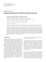
Figure 1: The flow graph of AAN n = 8.
actually be calculated by t − s additions and t − s shifts of
a, b,anda + b,wheres denotes the amount of am
i
+ bn
i
equal to 0. Since w
1
and w
2
are constants, the values of
m
i
, n
i
(i = 0, 1, , t) can be known in advance. So the
optimal scheme of additions and shifts can be designed to
decrease the amount of operations.
Most algorithms of the fast IDCT and DCT only deal
with each separate multiplication using additions and shifts
but our proposed method implements the linear combi-
nations of multiplications via additions and shifts, which
remarkably simplifies the computational complexity.
2.2. Reformation of AAN Algorithm Based on the General
Method. The 1D IDCT flow graph of AAN fast algorithm

[2], when n
= 8, is shown in Figure 1, where the symbol ci
denotes cos(iπ/16), and the scale coefficients A
i
(i = 0, ,7)
aredefinedasfollows:
A
0
=
1
2
√
2
≈ 0.3535533906,
A
1
=
cos
(
7π/16
)
2sin
(
3π/8
)
−
√
2
≈ 0.4499881115,
A

2
=
cos
(
π/8
)
√
2
≈ 0.6532814824,
A
3
=
cos
(
5π/16
)
√
2+2cos
(
3π/8
)
≈ 0.2548977895,
A
4
=
1
2
√
2
≈ 0.3535533906,

A
5
=
cos
(
3π/16
)
√
2 −2cos
(
3π/8
)
≈ 1.2814577239,
A
6
=
cos
(
3π/8
)
√
2
≈ 0.2705980501,
A
7
=
cos
(
π/16
)

√
2+2sin
(
3π/8
)
≈ 0.3006724435.
(10)
We reform the above algorithm flow graph based on our
method described in Section 2. The new flow graph is shown
in Figure 2.
In Figure 2, the butterfly computational structures are
replaced with the formulas of T1andT2. TheformulasofT1
C4
C4
T1
−
−
−
−
−
−
−
−
−
−
−
−
−
−
Input b

Input b
Input a
T2
A
0
X(0)
A
4
X(4)
A
2
X(2)
A
6
X(6)
A
1
X(1)
A
5
X(5)
A
3
X(3)
A
7
X(7)
x(0)
x(1)
x(2)

x(3)
x(4)
x(5)
x(6)
x(7)
Figure 2: The revised flow graph of AAN n = 8.
and T2, corresponding with w
1
and w
2
,andoptimalschemes
of additions and shifts are given as follows:
T1
= a · cos

π
8

−
b · cos

3π
8

=
a ·w
1
− b ·w
2
,

(11)
where w
1
= cos(π/8) and w
2
= cos(3π/8).
Optimal schemes of additions and shifts are
x
1
= a −
(
a
 3
)
;
// B1 (0.111)
2
x
2
=
(
b
 3
)
+
(
b  7
)
;
// B2 (0.0010001)

2
x = x
1
+
(
a  4
)
−
(
x
1
 6
)
+
(
x
1
 14
)
;
// B1 (0.11101100100000111)
2
x
3
= x
2
−
(
x
2

 10
)
+
(
b  2
)
;
// B2 (0.01100001111101111)
2
x = x − x
3
;
(12)
8 additions and 8 shifts are used in the step to implement the
computation of T1.
In the codes, x, x
1
, x
2
,andx
3
are all variables, and
symbol “
” denotes the right-shift operator. The binary
numbers B1 and B2 following the codes are the coefficients
of Input a and Input b, respectively. The result of each code
line can be expressed with B1, B2, a,andb.Nowweexplain
this step in details.
Factors w
1

and w
2
can be expressed as binary numbers.
Considering the precision and complexity of the computa-
tion,wechoose2
17
as the denominators, then
w
1
= cos

π
8

≈
121095
131072
= (0.11101100100000111)
2
,
w
2
= cos

3π
8

≈
50159
131072

= (0.01100001111101111)
2
.
(13)
When Input a is right-shifted r bits, the value is equal to 2
−r
·
a. So the code “x
1
= a − (a  3);” can be expressed by
mathematic expression as follows:
x
1
= a − 2
−3
· a =

1 −2
−3

· a = (0.111)
2
· a. (14)
4 EURASIP Journal on Advances in Signal Processing
So the binary number B1 following the code as the coefficient
of Input a is equal to (0.111)
2
.
In the same way, the code “x
2

= (b  3) + (b  7);”
means
x
2
= 2
−3
· b +2
−7
· b
=

2
−3
+2
−7

·
b
= (0.0010001)
2
· b.
(15)
The binary number B2 is equal to (0.0010001)
2
.
Then these codes implement the computation of T1:
x
= (0.11101100100000111)
2
· a

− (0.01100001111101111)
2
· b
= w
1
· a − w
2
· b.
(16)
With the similar method, we implement the computations of
T2and
√
2/2:
T2
= a × cos

3π
8

+ b ×cos

π
8

=
a ×w
1
+ b ×w
2
,

(17)
where w
1
= cos(3π/8) and w
2
= cos(π/8).
Optimal schemes of additions and shifts are
x
1
= b −
(
b
 3
)
;
// B2 (0.111)
2
x
2
=
(
a
 3
)
+
(
a  7
)
;
// B1 (0.0010001)

2
x = x
1
+
(
b  4
)
−
(
x
1
 6
)
+
(
x
1
 14
)
;
// B2 (0.11101100100000111)
2
x
3
= x
2
−
(
x
2

 10
)
+
(
a  2
)
;
// B1 (0.01100001111101111)
2
x = x + x
3
;
(18)
8 additions and 8 shifts are used in the step to implement the
computation of T2:
√
2
2
≈
46341
65536
= (0.1011010100000101)
2
. (19)
Optimal schemes of additions and shifts are
x
1
= a +
(
a  2

)
; // (1.01)
2
x
2
= x
1
 2; // (0.0101)
2
x
3
= a − x
2
; // (0.1011)
2
x
4
= x
1
+
(
x
2
 6
)
; // (1.0100000101)
2
x = x
3
+

(
x
4
 6
)
; // (0.1011010100000101)
2
.
(20)
In these codes, x, x
1
, x
2
,andx
3
are all variables, a is the
input, and the output is approximately equal to
√
2/2 ·
a. 4 additions and 4 shifts are used to implement the
computation of each
√
2/2, and 8 additions and 8 shifts are
needed to implement overall computations of
√
2/2 in the
1D IDCT computation. The computational complexity of 1D
IDCT is tabulated in Ta bl e 1 .
Table 1: The statistics of computational complexity.
Additions Shifts

Outside 26 0
T18 8
T28 8
√
2/28 8
Total1D 26+8+8+8
= 50 8+8+8= 24
−
−
−
−
−
−
−
−
−
−
−
−
−
−
−
C2
C2
C6
C6
C4
C4
h(6)
h(7)

g(6)
g(7)
A
0
X(0)
A
4
X(4)
A
2
X(2)
A
6
X(6)
A
1
X(1)
A
5
X(5)
A
3
X(3)
A
7
X(7)
x(0)
x(1)
x(2)
x(3)

x(4)
x(5)
x(6)
x(7)
Figure 3: The revised flow graph of AAN based on the character,
n
= 8.
Table 2: The statistics of computational complexity.
Additions Shifts
Outside 28 0
T15 6
T25 6
√
2/28 8
Total1D 28+5+5+8
= 46 6+6+8= 20
For the 1D IDCT, the total number of additions and shifts
is 50 and 24, respectively.
2.3. Rev ision Based on the Characteristics of AAN Algorithm.
Obviously, Input a and Input b in Figure 2 are computed
twice, in order to reduce the redundancy, another algorithm
is presented in Figure 3.
Details of the implementation of Figure 3 are presented
as follows
h
(
6
)
= g
(

7
)
× cos

π
8

−
g
(
6
)
× cos

3π
8

=
t
d
− t
a
,
h
(
7
)
= g
(
6

)
× cos

π
8

+ g
(
7
)
× cos

3π
8

=
t
b
+ t
c
,
(21)
where t
a
= g(6) × cos(3π/8), t
b
= g(6) × cos(π/8), t
c
=
g(7) × cos(3π/8), and t

d
= g(7) × cos(π/8). We also deal
with the computations of h(6) and h(7) with the similar
method introduced in Section 2.2 and choose 2
17
as the
denominators again.
EURASIP Journal on Advances in Signal Processing 5
S
S
0
S
1
16 8
8
x
x
0
x
1
buf1
buf0
Figure 4: The standard storage data structure.
Optimal schemes of additions and shifts are
t
1
= g
(
6
)

−

g
(
6
)
 4

; // (0.1111)
2
t
2
= t
1
+

g
(
6
)
 3

; // (1.0001)
2
t
3
= t
1
+
(

t
2
 10
)
; // (0.11110000010001)
2
t
a
=

g
(
6
)
 1

−
(
t
3
 3
)
; // (0.01100001111101111)
2
t
b
= t
3
−
(

t
1
 6
)
; // (0.11101100100001)
2
t
1
= g
(
7
)
−

g
(
7
)
 4

; // (0.1111)
2
t
2
= t
1
+

g
(

7
)
 3

; // (1.0001)
2
t
2
= t
1
+
(
t
2
 10
)
; // (0.11110000010001)
2
t
c
=

g
(
7
)
 1

−
(

t
3
 3
)
; // (0.01100001111101111)
2
t
d
= t
3
−
(
t
1
 6
)
; // (0.11101100100001)
2
h
(
6
)
= t
d
− t
a
;
h
(
7

)
= t
b
+ t
c
.
(22)
In order to reduce the computational complexity, we let
w
1
= cos

π
8

≈
121096
131072
= (0.11101100100001)
2
(23)
instead of
w
1
= cos

π
8

≈

121095
131072
= (0.11101100100000111)
2
.
(24)
The computational complexity of the improved method is
tabulated in Tab le 2.
For the 1D IDCT, the total number of additions and shifts
is 46 and 20, respectively.
3. Implementation of 2D IDCT
Inordertoimplementan8× 82DIDCTdefinedin(3),
we decompose it into a cascade of 1D IDCTs which are
applied to each row and column in the 8
×8IDCTcoefficient
matrix. The algorithm of 1D IDCT has been discussed
in Section 2. In this section, we will focus on the scale
coefficients A
i
(i = 0, , 7) and the matrices derived from
them which remarkably affect the computational precision
of the algorithm.
3.1. Choice of Coefficient Matrices and Compensation Matri-
ces. To ensure the precision of the transform, we use a
coefficient matrix and a compensation matrix to scale the
input X(n, m)(n, m
= 0, , 7) in the preprocessing. The
details are given as follows.
p
1

and p
2
are defined as scale factors, and coef[i][ j]
(i, j
= 0, 1, , 7) denotes the original floating-point matrix.
coef[i][j]isdefinedas
coef
[
i
]

j

=
A
i
× A
j
. (25)
Because the input data are multiplied by floating-point
matrix coef[i][ j], we just scale the floating-point matrix
coef[i][j]by2
p
1
to obtain integer coefficient matrix
coef0[i][ j] which is suitable for fixed-point computa-
tion. Considering rounding of fixed-point matrix, matrix
coef0[i][ j]ispresentedas
coef
[

i
]

j

=
coef
[
i
]

j

×
(
1
 P
1
)
,
coef0
[
i
]

j

=
(
int

)

coef
[
i
]

j

+0.5

.
(26)
In order to improve the computational precision, we expect
p
1
as greater as possible. However, the value of p
1
is limited
by the bit width of register. So we use the compensation
matrix coef1[i][j] to improve the precision of computations.
The compensation matrix is obtained as
coef
[
i
]

j

=

coef
[
i
]

j

− coef0
[
i
]

j

,
coef1
[
i
]

j

=
(
int
)

coef
[
i

]

j

×
(
1
 P
2
)
+0.5

.
(27)
Since the compensation matrix coef1[i][ j]storesp
2
-bit data
information, in some extent, the introduction of coef1[i][j]
improves p
2
-bit precision of the computations.
Matrix block[i][j](i, j
= 0, 1, ,7)isdefinedasan8×8
coefficient matrix. Then the preprocessing can be expressed
with the compensation matrix coef1[i][j] as follows:
block
[
i
]


j

= block
[
i
]

j

× coef0
[
i
]

j

+

block
[
i
]

j

× coef1
[
i
]


j

 P
2

.
(28)
Considering proper rounding at the final stage of the
transform, we add 2
p
1
−1
to all output data and right-shift
them by p
1
bits. Observing Figure 3 the flow graph of 1D
IDCT algorithm, we find that if we add 2
t
to X(0), then all
output x(k, l)(k, l
= 0, ,7) arealladdedby2
t
.Sowejust
need to add a bias 2
p
1
−1
to DC term X(0, 0):
block
[

0
][
0
]
= block
[
0
][
0
]
+
(
1 
(
P
1
− 1
))
, (29)
and simply right-shift all output x(k, l)(k, l
= 0, ,7)by p
1
bits for rounding of the 2D IDCT.
3.2. Implementation for 32-Bit Hardware. For 8-bit DCT
coefficients, corresponding IDCT coefficients are at most 11-
bit data. Due to the additions in the flow-graph, for 32-bit
hardware implementation we let p
1
= 18, p
2

= 3, so we get
the coefficient matrix and compensation matrix as follows:
6 EURASIP Journal on Advances in Signal Processing
coef0
=
⎡
⎢
⎢
⎢
⎢
⎢
⎢
⎢
⎢
⎢
⎢
⎢
⎢
⎢
⎢
⎢
⎢
⎢
⎣
32768 41706 60547 23624 32768 118768 25080 27867
41706 53081 77062 30068 41706 151163 31920 35468
60547 77062 111877 43652 60547 219455 46341 51491
23624 30068 43652 17032 23624 85627 18081 20091
32768 41706 60547 23624 32768 118768 25080 27867
118768 151163 219455 85627 118768 430476 90901 101004

25080 31920 46341 18081 25080 90901 19195 21328
27867 35468 51491 20091 27867 101004 21328 23699
⎤
⎥
⎥
⎥
⎥
⎥
⎥
⎥
⎥
⎥
⎥
⎥
⎥
⎥
⎥
⎥
⎥
⎥
⎦
,
coef1
=
⎡
⎢
⎢
⎢
⎢
⎢

⎢
⎢
⎢
⎢
⎢
⎢
⎢
⎢
⎢
⎣
0 −23 3 0 0 −4 −1
−2322−20 2−2
32023002
3 222 3
−12−1
0
−23 3 0 0 −4 −1
000
−10000
−4202−4013
−1 −22−1 −10 3−2
⎤
⎥
⎥
⎥
⎥
⎥
⎥
⎥
⎥

⎥
⎥
⎥
⎥
⎥
⎥
⎦
.
(30)
After preprocessing, we process 64 coefficients according
to the flow graph shown in Figure 3 by row-column way.
Finally, we right-shift the output back to the original scale
as
block
[
i
]

j

=

block
[
i
]

j



18. (31)
The multiplications of the coefficient matrix and the com-
pensation matrix in (28) can also be implemented with the
method of shifts and additions.
There are positive and negative elements in the com-
pensation matrix coef1[i][ j]. The purpose of this kind of
design is to reduce the absolute values of these elements and
decrease the computational complexity. Due to the limited
space, the details of optimal schemes of additions and shifts
for all elements in the matrices are omitted.
4. Implementations of 2D IDCT for 24-Bit and
16-Bit Hardware
In Section 3, we implemented the 2D IDCT for 32-bit
hardware. However in some cases it cannot be applied. Take
mobile devices for example. The bit width of these devices
is not enough to complete a 32-bit computation. So we
present the implementations of IDCTs for 24-bit and 16-bit
hardware in this section.
4.1. Implementation for 24-Bit Hardware. To implement the
above algorithm in 24-bit frame with the same idea, let
p
1
= 11 and p
2
= 5, then get the coefficient matrix and
compensation matrix:
coef0
=
⎡
⎢

⎢
⎢
⎢
⎢
⎢
⎢
⎢
⎢
⎢
⎢
⎢
⎣
256 326 473 185 256 928 196 218
326 415 602 235 326 1181 249 277
473 602 874 341 473 1714 362 402
185 235 341 133 185 669 141 157
256 326 473 185 256 928 196 218
928 1181 1714 669 928 3363 710 789
196 249 362 141 196 710 150 167
218 277 402 157 218 789 167 185
⎤
⎥
⎥
⎥
⎥
⎥
⎥
⎥
⎥
⎥

⎥
⎥
⎥
⎦
,
coef1
=
⎡
⎢
⎢
⎢
⎢
⎢
⎢
⎢
⎢
⎢
⎢
⎢
⎢
⎣
0 −61−14 0 −4 −2 −9
−6 −10 2 −3 −6 −112 3
1 211 1161 9
−14 −31 2−14 −18 −1
0
−61−14 0 −4 −2 −9
−4 −116−1435 3
−2121 8 −25−1 −12
−939−1 −93−12 5

⎤
⎥
⎥
⎥
⎥
⎥
⎥
⎥
⎥
⎥
⎥
⎥
⎥
⎦
.
(32)
After preprocessing, we process 64 coefficients according
to the flow graph shown in Figure 3 by row-column way.
Finally, we right-shift the output back to the original scale
as
block
[
i
]

j

=
block
[

i
]

j


11. (33)
The computations of 1D IDCTs for 24-bit hardware and 32-
bit hardware are nearly the same. The only difference is just
the bit width.
4.2. Implementat ion for 16-Bit Hardware. Considering that
the IDCT coefficients are at most 11-bit data, it is impossible
to implement the IDCT within 16-bit width to satisfy the
practical requirement of precision just through modifying
the scale factors p
1
and p
2
.
EURASIP Journal on Advances in Signal Processing 7
S
16 16
31
S
0
S
1
buf1buf0
Figure 5: The storage data structure for preprocessing.
In order to complete calculations of the IDCT according

to Figure 3 within 16-bit width, we use a combination of two
bytes as a unit to deal with calculations. We denote two 16-
bit buffers as buf0 and buf1 to store the high 16 bits and low
8 bits of the original 24-bit datum, respectively, which can be
expressed formally as follows.
Let the original 24-bit datum as x, and the data stored in
buf0 and buf1 are x
0
and x
1
,respectively.Then
x
= x
0
· 2
8
+ x
1
. (34)
In order to use unique data structure to express data, we
define the standard storage format, in which x
0
and x
1
must
satisfy the equations as follows:
−32768 ≤ x
0
≤ 32767, 0 ≤ x
1

≤ 255. (35)
This process also can be demonstrated by Figure 4.
In Figure 4, S, S
0
,andS
1
are all sign bits, and S
0
= S and
S
1
= 0 when data are stored in the standard storage format.
Due to the limit of 16-bit width, we cannot implement
preprocessing according to (28). We also use a combination
of two bytes as a unit which contains 30 data bits and 1
sign bit, and the method of additions and shifts to deal with
calculations in preprocessing. The data structure is showed
in Figure 5.
Because there are 30 data bits, we do not need the
compensation matrix but we use a new coefficient matrix
coef
16[i][j], which is defined as follows:
coef
[
i
]

j

= coef

[
i
]

j

×
(
1
 P
)
,
coef
16
[
i
]

j

=
(
int
)

coef
[
i
]


j

+0.5

,
(36)
where p
= p
1
+ p
2
= 11 + 5 = 16. The coefficient matrix is
presented as follows:
coef
16 =
⎡
⎢
⎢
⎢
⎢
⎢
⎢
⎢
⎢
⎢
⎢
⎢
⎢
⎣
8192 10426 15137 5906 8192 29692 6270 6967

10426 13270 19266 7517 10426 37791 7980 8867
15137 19266 27969 10913 15137 54864 11585 12873
5906 7517 10913 4258 5906 21407 4520 5023
8192 10426 15137 5906 8192 29692 6270 6967
29692 37791 54864 21407 29692 107619 22725 25251
6270 7980 11585 4520 6270 22725 4799 5332
6967 8867 12873 5023 6967 25251 5332 5925
⎤
⎥
⎥
⎥
⎥
⎥
⎥
⎥
⎥
⎥
⎥
⎥
⎥
⎦
.
(37)
Then the preprocessing can be expressed as follows with the
new coefficient matrix coef
16[i][j]:
block
[
i
]


j

=
block
[
i
]

j

×
coef 16
[
i
]

j

,
block
[
i
]

j

=
block
[

i
]

j

 P
2
.
(38)
After preprocessing, we transform the data into standard
format mentioned above and complete the computation of
IDCT.
As discussed above, in fact the algorithm for 16-bit
hardware is theoretically the same as for 24-bit hardware;
therearejustsomedifferences in the implementations. In
other words, we complete the 24-bit computations within
16-bit width, so that we could gain the same precisions.
5. Performances of Our Proposed Algorithms
In order to evaluate the performances of the novel algorithm,
we test it referring to IEEE 1180 [13] and ISO/IEC 23002-
1[14] specifications. We use the specified pseudorandom
input matrices X
i
(Q denotes the testing quantity, i =
1, 2, , Q), test out our algorithm, and investigate five
metrics:
peak pixel err:
p
= max
k,l,i




x
i
(
k, l
)
− x
0
i
(
k, l
)


,
peak mean square err:
e
= max
k,l
⎡
⎣
1
Q
Q−1

i=0
(x
i

(k, l) − x
0
i
(k, l))
2
⎤
⎦
,
over mean square err:
n
=
1
64
7

k=0
7

l=0
⎡
⎣
1
Q
Q−1

i=0
(x
i
(k, l) − x
0

i
(k, l))
2
⎤
⎦
,
peak mean err:
d
= max
k,l
⎡
⎣
1
Q
Q−1

i=0
(
x
i
(
k, l
)
− x
0
i
(
k, l
))
⎤

⎦
,
over mean err:
m
=
1
64
7

k=0
7

l=0
⎡
⎣
1
Q
Q−1

i=0
(
x
i
(
k, l
)
− x
0
i
(

k, l
))
⎤
⎦
.
(39)
Here,
x
i
(k, l)(k, l = 0, , 7) denote the reconstructed
pixel values of the specified pseudorandom input matrices
X
i
,andx
0i
(k, l)(k, l = 0, , 7) denote reference values
correspondingly.
The IEEE 1180 indicates that these metrics must satisfy
these accuracy requirements: p
≤ 1, e ≤ 0.06, n ≤
0.02, d ≤ 0.015, and m ≤ 0.0015. The performances of our
proposed algorithm are presented in Tables 3 and 4.Because
computational precisions of the algorithms for 24-bit and 16-
bit hardware are the same, we just give one table to show the
results.
From the previous tables, it is obvious that the precisions
of IDCT for 24-bit and 16-bit hardware are lower than
8 EURASIP Journal on Advances in Signal Processing
Table 3: IDCT precision performance for 32-bit hardware.
Q L, H Negation p(ppe) ≤ 1 e(pmse) ≤ 0.06 n(omse) ≤ 0.02 d(pme) ≤ 0.015 m(ome) ≤ 0.0015

10 000 5, 5 No 1.000000 0.000300 0.000064 0.000300 0.000064
10 000 5, 5 Yes 1.000000 0.000400 0.000070 0.000400 0.000070
10 000 256, 255 No 1.000000 0.000800 0.000252 0.000400 0.000061
10 000 256, 255 Yes 1.000000 0.000800 0.000244 0.000500 0.000094
10 000 300, 300 No 1.000000 0.000800 0.000300 0.000500 0.000087
10 000 300, 300 Yes 1.000000 0.000700 0.000278 0.000400 0.000038
10 000 384, 383 No 1.000000 0.000700 0.000234 0.000400 0.000022
10 000 384, 383 Yes 1.000000 0.000800 0.000238 0.000400 0.000034
10 000 512, 511 No 1.000000 0.000600 0.000231 0.000400 0.000022
10 000 512, 511 Yes 1.000000 0.000600 0.000241 0.000400 0.000031
1 000 000 5, 5 No 1.000000 0.000105 0.000064 0.000105 0.000064
1 000 000 5, 5 Yes 1.000000 0.000115 0.000067 0.000115 0.000067
1 000 000 256, 255 No 1.000000 0.000332 0.000256 0.000116 0.000062
1 000 000 256, 255 Yes 1.000000 0.000347 0.000255 0.000115 0.000064
1 000 000 300, 300 No 1.000000 0.000348 0.000252 0.000107 0.000054
1 000 000 300, 300 Yes 1.000000 0.000357 0.000253 0.000118 0.000056
1 000 000 384, 383 No 1.000000 0.000331 0.000241 0.000080 0.000042
1 000 000 384, 383 Yes 1.000000 0.000324 0.000239 0.000095 0.000042
1 000 000 512, 511 No 1.000000 0.000307 0.000236 0.000081 0.000034
1 000 000 512, 511 Yes 1.000000 0.000310 0.000232 0.000061 0.000032
Table 4: IDCT precision performance for 24-bit or 1-bit hardware.
Q L, H Negation p(ppe) ≤ 1 e(pmse) ≤ 0.06 n(omse) ≤ 0.02 d(pme) ≤ 0.015 m(ome) ≤ 0.0015
10 000 5, 5 Yes 1.000000 0.001300 0.000558 0.001000 0.000098
10 000 5, 5 No 1.000000 0.001500 0.000603 0.001500 0.000184
10 000 256, 255 Yes 1.000000 0.013600 0.008787 0.002700 0.000066
10 000 256, 255 No 1.000000 0.013400 0.008839 0.002300 0.000114
10 000 300, 300 Yes 1.000000 0.014700 0.008817 0.002400 0.000061
10 000 300, 300 No 1.000000 0.014700 0.008787 0.002100 0.000244
10 000 384, 383 Yes 1.000000 0.014600 0.008742 0.003400 0.000092
10 000 384, 383 No 1.000000 0.014600 0.008763 0.002100 0.000003

10 000 512, 511 Yes 1.000000 0.011800 0.008511 0.002500 0.000005
10 000 512, 511 No 1.000000 0.012900 0.008586 0.001800 0.000052
10 00000 5, 5 Yes 1.000000 0.001242 0.000559 0.001242 0.000139
10 00000 5, 5 No 1.000000 0.001292 0.000561 0.001292 0.000141
10 00000 256, 255 Yes 1.000000 0.012672 0.008839 0.001420 0.000125
10 00000 256, 255 No 1.000000 0.012660 0.008839 0.001189 0.000119
10 00000 300, 300 Yes 1.000000 0.012367 0.008761 0.001123 0.000103
10 00000 300, 300 No 1.000000 0.012380 0.008753 0.001069 0.000094
10 00000 384, 383 Yes 1.000000 0.012075 0.008641 0.000921 0.000070
10 00000 384, 383 No 1.000000 0.012136 0.008649 0.000771 0.000068
10 00000 512, 511 Yes 1.000000 0.012110 0.008620 0.000875 0.000020
10 00000 512, 511 No 1.000000 0.012138 0.008620 0.000663 0.000055
the precision of IDCT for 32-bit hardware but still meet
corresponding specifications very well [11, 12].
We estimate the implementation costs of our algo-
rithm in Tabl e 5 in terms of 1D and 2D computational
complexities. The 1D computational complexity means the
complexity of executing our 8-point IDCT algorithm, and
the 2D computational complexity includes the computations
of 16 iterations of 1D IDCTs, an addition for rounding and
the right shifts at the end of the transform.
In many image and video Codecs, it is also possible
to simply merge factors involved in IDCT scaling with
the factors used by the corresponding inverse-quantization
EURASIP Journal on Advances in Signal Processing 9
Table 5: Computational complexities of 1D and 2D IDCT.
Additions Shifts
1D IDCT 46 20
2D IDCT 737 384
process. In such cases, scaling can be executed without taking

any extra resources. So we do not take account of these
computational complexities in Tab le 5.
6. Conclusions
In this paper, we propose a new general method to compute
the fast IDCT, which can be applied to most existing IDCT
algorithms with butterfly computational structures. We also
introduce a specific algorithm derived from AAN algorithm.
Considering characteristics of the AAN algorithm, coefficient
matrices and compensation matrices are brought into the
algorithm to improve its precision. Through varying the
scale coefficients p
1
and p
2
, we can modify the precision
to meet the different requirements of hardware, such as
32-bit hardware and 24-bit hardware. However, in order
to implement our algorithm using 16-bit hardware with
satisfied precision, we have to revise our design which
includes a new coefficient matrix, a new kind of data
structure, and some new methods of data manipulation.
The new IDCT algorithm achieves a good compromise
between the precision and computational complexity. The
idea of optimizing the IDCT algorithm can also be extended
to other similar fast algorithms.
Acknowledgments
This work was supported partly by NSFC under Grants
60672060, the Research Fund for the Doctoral Program of
Higher Education, and HiSilicon Technologies Co. Ltd.
References

[1] B. Lee, “A new algorithm to compute the discrete cosine
transform,” IEEE Transactions on Acoustics, Speech, and Signal
Processing, vol. 32, no. 6, pp. 1243–1245, 1984.
[2] Y. Arai, T. Agui, and M. Nakajima, “A fast DCT-SQ scheme for
images,” Transactions of the IEICE, vol. 71, no. 11, pp. 1095–
1097, 1988.
[3] C. Loeffler, A. Ligtenberg, and G. S. Moschytz, “Practical fast
1-D DCT algorithms with 11 multiplications,” in Proceedings
of the IEEE International Conference on Acoustics, Speech, and
Signal Processing (ICASSP ’89), vol. 2, pp. 988–991, Glasgow,
UK, May 1989.
[4] A. Elnaggar and H. M. Alnuweiri, “A new multidimensional
recursive architecture for computing the discrete cosine
transform,” IEEE Transactions on Circuits and Systems for Video
Technology, vol. 10, no. 1, pp. 113–119, 2000.
[5] L P. Chau and W C. Siu, “Recursive algorithm for the
realization of the discrete cosine transform,” in Proceedings
of the IEEE International Symposium on Circuits and Systems
(ISCAS ’00), vol. 5, pp. 529–532, Geneva, Switzerland, May
2000.
[6] C H. Chen, B D. Liu, J F. Yang, and J L. Wang, “Efficient
recursive structures for forward and inverse discrete cosine
transform,” IEEE Transactions on Signal Processing, vol. 52, no.
9, pp. 2665–2669, 2004.
[7] C H. Chen, B D. Liu, and J F. Yang, “Condensed recursive
structures for computing multidimensional DCT/IDCT with
arbitrary length,” IEEE Transactions on Circuits and Systems I,
vol. 52, no. 9, pp. 1819–1831, 2005.
[8] J. Lee, N. Vijaykrishnan, and M. J. Irwin, “Inverse discrete
cosine transform architecture exploiting sparseness and sym-

metry properties,” IEEE Transactions on Circuits and Systems
for Video Technology, vol. 16, no. 5, pp. 655–662, 2006.
[9] J S. Chiang, Y F. Chiu, and T H. Chang, “A high throughput
2-dimensional DCT/IDCT architecture for real-time image
and video system,” in Proceedings of the 8th IEEE International
Conference on Electronics, Circuits and Systems (ICECS ’01),
vol. 2, pp. 867–870, Msida, Malta, September 2001.
[10] R. Kutka, “Fast computation of DCT by statistic adapted look-
up tables,” in Proceedings of the IEEE International Conference
on Multimedia and Expo (ICME ’02), vol. 1, pp. 781–784,
Lausanne, Switzerland, August 2002.
[11] T. D. Tran, “The binDCT: fast multiplierless approximation of
the DCT,” IEEE Signal Processing Letters, vol. 7, no. 6, pp. 141–
144, 2000.
[12] J. Liang and T. D. Tran, “Fast multiplierless approximations of
the DCT with the lifting scheme,” IEEE Transactions on Signal
Processing, vol. 49, no. 12, pp. 3032–3044, 2001.
[13] CAS Standards Committee of the IEEE Circuits and Systems
Society, “IEEE standard specifications for the implementa-
tions of 8
× 8 inversediscrete cosine transform,” March 1991.
[14] ISO/IEC 23002-1:2006, JTC1/SC29/WG11 N7815, “Informa-
tion technology—MPEG video technologies—part 1: accu-
racy requirements for implementation of integer-output 8
× 8
inverse discrete cosine transform”.