Differential Neural Networks Observers: development, stability analysis and implementation

73
0 0.2 0.4 0.6 0.8 1 1.2 1.4 1.6 1.8 2
-1.5
-1
-0.5
0
0.5
1
1.5
2
2.5
x 10
-3
Time [s]
mole
x
3
min
x
3
DNN Observer without projection
x
3
Projectional DNN Observer
x
3

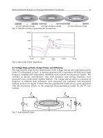
Figure 4. Estimation of x
3

(t) (2 s)






0 2 4 6 8 10 12 14 16 18 20
-2
-1
0
1
2
3
4
5
6
7
x 10
-3
Time [s]
mol e
x
3
x
3
Project ional DNN Observer
x
3
DNN Observer without projection


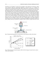
Figure 5. Estimation of x
3
(t) (20 s)
Systems, Structure and Control

74
0 0.1 0.2 0.3 0.4 0.5 0.6 0.7 0.8 0.9 1
-5
-4
-3
-2
-1
0
1
2
3
4
5
x 10
-4
Time [s]
g/g
soil
x
4
DNN Observer without projection
x
4
Projectional DNN Observer

x
4
x
4
min
x
4
max

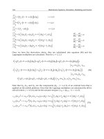
Figure 6. Estimation of x
4
(t) (1 s)



0 0.5 1 1.5 2 2.5 3 3.5 4 4.5 5
-5
-4
-3
-2
-1
0
1
2
3
4
5
x 10
-4
Ti me [ s]

g/g
soil
x
4

x
4
Project ional DNN Observer
x
4
DNN Observer without projection

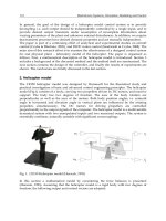
Figure 7. Estimation of x
4
(t) (5 s)
As it can be seen, the projectional DNNO has significantly better quality in state estimation,
especially in the beginning of the process, when negative values and over-estimation have
been obtained by a non-projectional DNNO.
Differential Neural Networks Observers: development, stability analysis and implementation

75
6. Conclusion and future work
The complete convergence analysis for this class of adaptive observer is presented. Also the
boundedness property of the adaptive weights in DNN was proven. Since the projection
method leads to discontinuous trajectories in the estimated states, a nonstandard Lyapunov
- Krasovski functional is applied to derive the upper bound for estimation error (in "average
sense"), which depends on the noise power (output and dynamics disturbances) and on an
unmodelled dynamic. It is shown that the asymptotic stability is attained when both of these
uncertainties are absent. The illustrative example confirms the advantages, which the
suggested observers have being compared with traditional ones.

Appendix (proof of Theorem 2)
Evidently that
()
() ()
)tht(tLhtt −−
′
≤−−
′
δ
δδ

() () ()
ηη
η
η
η
η
ηη
η
η
η
ϒ
−
Λ≤
Λ
−
Λ
≤
⎟
⎠

⎞
⎜
⎝
⎛
Λ
−
ΛΛ=
21
1
2
1
21121
/
)t(
t
/
,t
/
t

ξξ
ξ
ϒ
−
Λ≤
21
1
/
)t(
()

21
2
1
10
21
1
/
f
~
txf
~
f
~
/
f
~
)t(f
~
⎥
⎥
⎥
⎦
⎤
⎢
⎢
⎢
⎣
⎡
Λ
+

−
Λ≤

where
() () ()
txtx
ˆ
:tδ
′
−
′
=
′
is the state estimation error at time
t
.
Consider the next "nonstandard" Lyapunov-Krasovskii ("energetic") function
()
() () ()
{}
τ
dτW
~
τ
T
W
~
trτk
p
δ(τ)

t
tht
V(t)
⎥
⎦
⎤
⎢
⎣
⎡
+
∫
−
=
2

where
.W
ˆ
W(τ((ττ)W
~
−= Since the problem under consideration contains uncertainties and
external output disturbances we won't demonstrate that the time-derivative of this energetic
function is strictly negative. Instead, we will use it to obtain an upper bound for the
averaged state estimation error. Taking time derivative of Lyapunov-Krasovski function and
considering the property (5), the assumption
A2, and in view of (29) we have:
Systems, Structure and Control

76
()

() ()
[]
()
() () ()
{}
()
()
()
()
{}
() () ()
{}
()
()
()
()
{}
()
() ()
[]
()
() ( )
[]
()
() () ()
{}
()
()
()
()

{}
() () ()
{}
()
()
()
()
{}
)
)(+W
ˆ
+W
ˆ
+x
++++
)
t
)(x-
)x
ˆ
x
ˆ
tht(W
~
)tht(W
~
thtktW
~
tW
~

tk
)tht(W
~
)tht(W
~
thtktW
~
tW
~
tk
tht-d)()(f
~
)(u)(x()t(x)t(Ax-))t(h-t(
d))(C-)((K)(u)(x
ˆ
)((W)(x
ˆ
)(W)(x
ˆ
A))t(h-t(x
ˆ
tht(W
~
)tht(W
~
thtktW
~
tW
~
tk

)tht(W
~
)tht(W
~
thtktW
~
tW
~
tk
)ht(
p
t
d))t(x
ˆ
C-)(+)(Cx(K+)(u
)()((W+)()(W+)(x
ˆ
A
t
ht
+))t(h-t(x
ˆ
)t(V
dt
d
TT
TT
p
p
t

tht
t
tht
TT
TT
p
t
X
−−−−+
−−−−+
−+
≤−−−−
+−−−−
+−
−
−=
≤
−=
−=
∫−
∫
⎪
⎭
⎪
⎬
⎫
⎪
⎩
⎪
⎨

⎧
∫
222222
111111
2
2
21
21
222222
111111
2
2
21
trtr
trtr
trtr
trtr
δττξτττϕσ
ττδτηττϕττσττ
δ
ττητττϕττσττ
τ
π
τ
τ

Taking into account that
()
bPa,
P

b
P
a
P
ba 2
222
++=+
Defining:
()()
()()
x(t)(t)x
ˆ
:(t)
~
x(t)σ(t)x
ˆ
σ(t):σ
~
, i
i
W
ˆ
(t)
i
W(t):
i
W
~
KC,A:A
~

ϕϕϕ
−=
−=
=−=
−=
21

we derive
() ()
() () ()
{}
()() () ()
{}
() () ()
{}
()() () ()
{}
)th(tW
~
)th(t
T
W
~
trthtktW
~
t
T
W
~
trtk

)th(tW
~
)th(t
T
W
~
trthtktW
~
t
T
W
~
trtk
tβtαV
−−−−
+−−−−
++≤
222222
111111


where:
()
()
() ()
[
]
() ( )
()
() ()

[
]
)
τττξτηττϕ
ττϕττστσττδ
τ
δβ
τττξτηττϕ
ττϕττστσττδ
τ
α
d)(f
~
)()(K)(u)(
~
W
ˆ
)(u)(x
ˆ
)((W
~
)(
~
W
ˆ
)(x
ˆ
)(W
~
)(A

~
t
tht
,htP:t
P
d)(f
~
)()(K)(u)(
~
W
ˆ
)(u)(x
ˆ
)((W
~
)(
~
W
ˆ
)(x
ˆ
)(W
~
)(
A
~
t
tht
:t
−−++

⎜
⎜
⎝
⎛
+++
∫
−=
−=
−−+
++++
∫
−=
=
2
211
2
2
2
211

Differential Neural Networks Observers: development, stability analysis and implementation

77
The term
()
tβ is expanded as
() ()()
()
()
()()

()
() () ()()
()
()
()()
()
()
()()
()
()()
()
() ()() ()()
()
()
⎟
⎟
⎠
⎞
⎜
⎜
⎝
⎛
∫
−=
−−
⎟
⎟
⎠
⎞
⎜

⎜
⎝
⎛
−
∫
−=
−+
⎟
⎟
⎟
⎠
⎞
⎜
⎜
⎜
⎝
⎛
∫
−=
−+
⎟
⎟
⎠
⎞
⎜
⎜
⎝
⎛
∫
−=

−+
⎟
⎟
⎠
⎞
⎜
⎜
⎝
⎛
∫
−=
−+
⎟
⎟
⎠
⎞
⎜
⎜
⎝
⎛
∫
−=
−
+
⎟
⎟
⎠
⎞
⎜
⎜

⎝
⎛
∫
−=
−=
ττ
τ
δττξτη
τ
δ
τττϕ
τ
δ
τττϕτ
τ
δ
ττσ
τ
δττστ
τ
δ
ττδ
τ
δβ
df
~
t
tht
,thtPdK
t

tht
,thtP
d)(u)(
~
W
ˆ
t
tht
,thtP
d)(u)(x
ˆ
)((W
~
t
tht
,thtP
d
~
W
ˆ
t
tht
,thtPdx
ˆ
W
~
t
tht
,thtP
dA

~
t
tht
,thtP
t
22
2
2
2
2
2
1
22
2

Similarly, we can estimate
t
α
by the Jensen's inequality we get
()
()
() ()
[
]
()
() () ()
()
() () ()
⎪
⎭

⎪
⎬
⎫
⎟
⎟
⎠
⎞
⎜
⎜
⎝
⎛
+++
∫
−=
+
⎪
⎩
⎪
⎨
⎧
⎟
⎟
⎠
⎞
⎜
⎜
⎝
⎛
+++
∫

−=
≤−−++
+++
∫
−=
=
ττξττηττϕ
τ
τττϕττστσττδ
τ
τττξτηττϕ
ττϕττστσττδ
τ
α
d
p
p
f
~
p
K
p
)(u)(
~
W
ˆ
t
tht
d
p

)(u)(x
ˆ
)((W
~
p
)(
~
W
ˆ
p
)(x
ˆ
)(W
~
p
A
~
t
tht
P
d)(f
~
)()(K)(u)(
~
W
ˆ
)(u)(x
ˆ
)((W
~

)(
~
W
ˆ
)(x
ˆ
)(W
~
)(A
~
t
tht
:t
2
2
2
2
2
2
2
2
1
2
1
2
8
2
2
211


Each term of
t
α
and )t(
β
is upper bounded, next facts are used. Norm inequality AB ≤
BA and the matrix inequality
T
Y
Y
Λ
T
X
Λ
Λ
T
Y
X
T
X
Y
1−
+≤+

valid for any
sr
RYX,
×
∈ and any
ssT

RΛΛ
×
∈=<0 (Poznyak, 2001).
It also necessary to represents the state estimation error
t
δ
as a function of the available
output, the estimation error
t
e :
() () () () () ()
() () ()()
() () () () ()
() () () ()
tIC
T
Ctt
T
Cte
T
C
tttC
T
Ct
T
Cte
T
C
ttC
T

Cte
T
C
ttCxtx
ˆ
Ctyty
ˆ
te
δϖϖδη
ϖδϖδδη
ηδ
η
⎟
⎠
⎞
⎜
⎝
⎛
+=++−
−+=+−
−=−
−−=−=−

Giving
() () () ()
⎟
⎠
⎞
⎜
⎝

⎛
++−= tt
T
Cte
T
CNt
ϖδη
ϖ
δ

Systems, Structure and Control

78
where:
1−
⎟
⎠
⎞
⎜
⎝
⎛
+= IC
T
C:N
ϖ
ϖ

and
ϖ
is a small positive scalar. Taking into account all these facts next estimation is

obtained:
()
()
() ( )
()
+
−
⎥
⎦
⎤
+
⎟
⎠
⎞
⎜
⎝
⎛
−
+
−
+
⎟
⎠
⎞
⎜
⎝
⎛
ϒ+++ϒ+
⎟
⎠

⎞
+
⎟
⎠
⎞
⎜
⎝
⎛
−
+
−
+
−
+
−
+
−
⎢
⎣
⎡
++
−
≤
tht
δQΛΛIL
u
μ
σ
Lμμ
u

LΛ
σ
LΛ
PΛΛ
T
W
ˆ
ΛW
ˆ
T
W
ˆ
ΛW
ˆ
ΛP
A
~
PP
T
A
~
T
t
ht
δth)t(V
dt
d
0
1
7

1
3
2
321
2
85
1
10
1
92
1
821
1
51
1
1
ϖ
ϕϕ


()
()
() ()
()
()
()
() ()()
()
()() ()
()

() ()()
dττx
ˆ
στW
~
PNΛCCΛPNτ
T
W
~
τx
ˆ
T
σ
t
thtτ
dττx
ˆ
στW
~
PCNtht
T
e
t
thtτ
tht
δQ
T
tht
δ
ηξξ

ΛP
Diam(x)
f
~
Λf
~
f
~
f
~
ΛP
η
/
η
ΛPK
f
~
Λ
txf
~
f
~
f
~
ΛΛ
ξ
/
ξ
Λ
η

/
η
ΛKΛh(t)
δ
L
u
L
Λ
δ
LL
u
μ
δ
L
μ
δ
L
σ
L
μ
δ
L
σ
L
Λ
δ
L
A
~
Λth

⎥
⎦
⎤
⎢
⎣
⎡
+
∫
−=
+
⎟
⎠
⎞
⎜
⎝
⎛
−
∫
−=
+
⎥
⎦
⎤
−−
−ϒ+ϒ
−
⎟
⎟
⎠
⎞

+
⎥
⎦
⎤
⎢
⎣
⎡
+
−
+ϒ
−
⎢
⎢
⎢
⎣
⎡
+
⎥
⎥
⎥
⎦
⎤
⎢
⎢
⎢
⎣
⎡
+
−
+

⎟
⎟
⎠
⎞
⎜
⎜
⎝
⎛
⎟
⎟
⎠
⎞
⎜
⎜
⎝
⎛
ϒ
−
+ϒ
−
+
⎥
⎥
⎥
⎦
⎤
⎢
⎢
⎢
⎣

⎡
ϒ
+
ϒ
++++
1321
1
2
0
2
1
21
10
1
21
1
2
2
1
10
1
10
2
21
1
21
1
9
3
22

8
3
22
3
3
2
1
3
2
2
3
2
5
4
2
2
1
3
ϖ
ϖ
ϖ
ϖ
ϕϕ


()
() ()
() () ()
{}
()() () ()

{}
()
()
()
()
()
()() () ( )
()
() ()
() () ()
{}
()() () ()
{}
)th(t
2
W
~
)th(t
T
2
W
~
trtht
2
kt
2
W
~
t
T

2
W
~
trt
2
k
)dτu()(x
ˆ
)((
2
W
~
)P(
T
2
W
~
T
)(x
ˆ
)((
T
u
t
thtτ
)dτu()(x
ˆ
)((
2
W

~
PN
7
ΛC
6
Λ
T
CPNτ
T
2
W
~
τx
ˆ
T
)(
T
u
t
thtτ
dτ)u()(x
ˆ
)((
2
W
~
PCNtht
T
e2
t

thtτ
)th(t
1
W
~
)th(t
T
1
W
~
trtht
1
k
t
1
W
~
t
T
1
W
~
trt
1
kdτ
τ
x
ˆ
σ
τ

W
~
)P(
T
1
W
~
τ
x
ˆ
T
σ
t
thtτ
−−−−
+
∫
−=
+
⎟
⎠
⎞
⎜
⎝
⎛
+
∫
−=
+
⎟

⎠
⎞
⎜
⎝
⎛
−
∫
−=
+−−−
−+
∫
−=
+
ττϕτττϕτ
ττϕτ
ϖ
ϖ
ϖ
ϕτ
ττϕτ
ϖ
τ


Differential Neural Networks Observers: development, stability analysis and implementation

79
Considering
() ()
()

() ( )
()
0
1
7
1
3
2
321
2
85321
1
10
1
92
1
821
1
51
1
1
1
0
321
1
Q
IL
u
L
u

LL,,,Q
T
W
ˆ
W
ˆ
T
W
ˆ
W
ˆ
R
,,,QPPRKA
~
PPK
T
A
~
+
⎟
⎠
⎞
⎜
⎝
⎛
−
Λ+
−
Λ+
⎥

⎦
⎤
⎢
⎣
⎡
ϒ+++ϒΛ+Λ=
−
Λ+
−
Λ+
−
Λ+
−
Λ+
−
Λ=
−
≤+
−
++
ϖ
ϕ
μ
σ
μμ
ϕσ
μμμδ
μμμδ

implies:

()
()
()
()
() ()()
() ()()
]
()()
}
() () ()
{}
()( ) () ()
{}
0
111111
1
123
2
1
=−−−−+
+
⎩
⎨
⎧
⎢
⎣
⎡
⎟
⎠
⎞

⎜
⎝
⎛
Λ+Λ+−
∫
−=
)tht(W
~
)tht(
T
W
~
trthtktW
~
t
T
W
~
trtk
dx
ˆ
T
x
ˆ
W
~
x
ˆ
W
~

PNC
T
CNthte
T
CNP
T
W
~
tr
t
t
ht
ττστστ
τστ
ϖ
ϖ
ϖϖ
τ
τ

that can be obtained selecting
()
()
()
() ()()
() ()()
]
()()
()
⎭

⎬
⎫
−
⎩
⎨
⎧
⎢
⎣
⎡
⎟
⎠
⎞
⎜
⎝
⎛
−
=
tW
~
dt
(t)dk
τx
ˆ
T
στx
ˆ
στW
~
+τx
ˆ

στW
~
PNCΛ
T
+CΛ+Ntt-he
T
CNP
(t)k
-
tW
dt
d
1
1
1
123
2
1
2
1
1
ϖ
ϖ
ϖϖ

Analogously, for the second adaptive law
()
()
()
()

() ( )
()
]
()()
}
() () ()
{}
()() () ()
{}
0
222222
2
176
2
2
=−−−−+
+
⎩
⎨
⎧
⎢
⎣
⎡
⎟
⎠
⎞
⎜
⎝
⎛
Λ+Λ+−

∫
−=
)tht(W
~
)tht(
T
W
~
thtktW
~
t
T
W
~
tk
dx
ˆ
T
)(
T
u)(u)(x
ˆ
)((W
~
)(u)(x
ˆ
(W
~
PNC
T

C
Nthte
T
CNP
T
W
~
t
tht
trtr
tr
ττϕτττϕτ
ττϕτ
ϖ
ϖ
ϖϖ
τ
τ

leading to
()
()
()
() ( )
()
]
()()
()
⎭
⎬

⎫
−
⎩
⎨
⎧
⎢
⎣
⎡
⎟
⎠
⎞
⎜
⎝
⎛
ΛΛ
−
−
=
tW
~
dt
)t(dk
x
ˆ
T
)(
T
u)(u)(x
ˆ
)((W

~
+)(u)(x
ˆ
(W
~
PN+C
T
CN+th-te
T
CNP
)t(k
tW
dt
d
2
2
2
176
2
1
2
2
2
τϕτττϕτ
ττϕτ
ϖ
ϖ
ϖϖ

Systems, Structure and Control


80
Finally:
()
()
() ()
⎥
⎦
⎤
−−
−ϒ+ϒ
−
Λ+
⎥
⎦
⎤
⎢
⎣
⎡
Λ+
−
Λ+ϒ
−
Λ+
⎢
⎢
⎢
⎣
⎡
⎥

⎥
⎥
⎦
⎤
⎢
⎢
⎢
⎣
⎡
Λ
+
−
ΛΛ+
⎟
⎟
⎠
⎞
⎜
⎜
⎝
⎛
⎟
⎟
⎠
⎞
⎜
⎜
⎝
⎛
ϒ

−
Λ+ϒ
−
ΛΛ+
⎥
⎥
⎥
⎦
⎤
⎢
⎢
⎢
⎣
⎡
ϒ
Λ+
ϒ
+++Λ+Λ≤
tht
Q
T
tht
P
)x(Diam
f
~
f
~
f
~

f
~
P
/
PK
f
~
txf
~
f
~
f
~
//
K)t(h
L
u
LLL
u
LLLLLL
A
~
th)t(V
dt
d
δδ
ηξξ
ηη
ξξηη
δϕδϕ

μ
δ
μ
δσ
μ
δσδ
0
2
1
21
10
1
21
1
2
2
1
10
1
10
2
21
1
21
1
9
3
22
8
3

22
3
3
2
1
3
2
2
3
2
5
4
2
2
1
3

or in the short form:
() ()
()
()
()
()
⎟
⎠
⎞
⎜
⎝
⎛
−−−+≤ thtQtht

T
bathth)t(V
dt
d
δδ
0
2

where
()
ηξξηη
ξξηη
δϕδϕ
μ
δ
μ
δσ
μ
δσδ
ϒ+ϒ
−
Λ+
⎥
⎦
⎤
⎢
⎣
⎡
Λ+
−

Λ+ϒ
−
Λ+
⎥
⎥
⎥
⎦
⎤
⎢
⎢
⎢
⎣
⎡
Λ
+
−
ΛΛ+
⎟
⎟
⎠
⎞
⎜
⎜
⎝
⎛
⎟
⎟
⎠
⎞
⎜

⎜
⎝
⎛
ϒ
−
Λ+ϒ
−
ΛΛ=
ϒ
Λ+
ϒ
+++Λ+Λ=
2
121
10
1
21
1
2
2
1
10
1
10
2
21
1
21
1
9

3
22
8
3
22
3
3
2
1
3
2
2
3
2
5
4
2
2
1
P)x(Diam
f
~
f
~
f
~
f
~
P
/

PK
f
~
txf
~
f
~
f
~
//
K:b
L
u
LLL
u
LLLLLL
A
~
:a

So,
()
()
()
()
()
(
)
()
thdt

)t(dV
btahthtQtht
T
1
2
0
−+≤−−
δδ

And integrating, we obtain
()
()
()
τ
τ
τ
τ
τττδττδ
τ
d
)(h
dt
)t(dV
b)(ah
T
d)(thQ)(h
T
T
⎥
⎦

⎤
⎢
⎣
⎡
−
⎟
⎠
⎞
⎜
⎝
⎛
+
=
∫≤−−
=
∫
1
2
0
0
0

And hence,
()
)(h
V
)(h
V
th
t

V
)(h
V
d
T
d)(h
)(h
V
T
+
)(h
V
d
T
-
)(h
dV
T
0
0
0
0
0
2
000
≤+−=
⎟
⎟
⎠
⎞

⎜
⎜
⎝
⎛
=
∫−
≤
=
∫
⎟
⎟
⎠
⎞
⎜
⎜
⎝
⎛
=
∫=
=
∫−
τ
τ
τ
ττ
τ
τ
τ
τ
τ

τ
τ
τ
τ

This implies
()
()
()
()
()
)(h
V
bTdthQ
T
ad)(th)(th
T
T
0
0
2
0
0
0
++≤∫
=
∫−−
=
ττδτδ
τ

τττ
τ

Dividing by
T
and taking the upper limit we finally get (30).
Differential Neural Networks Observers: development, stability analysis and implementation

81
8. References
Abdollahi, F. Talei, A., & Patel R. (2006). A stable neural network based observer with
application to flexible joint manipulators.
IEEE Transactions on Neural Networks. Vol
17. No 1 pp 118-129.
Alamo, T., Bravo, J. M. & Camacho, E. F. (2005). Guaranteed state estimation by zonotopes.
Automatica vol 41 pp 1035-1043.
Chairez, I., Poznyak, A. & Poznyak, T. (2006). New Sliding mode learning law for Dynamic
Neural Network Observer.
IEEE Transactions on Circuits Systems II. Vol 53. Pp 1338-
1342.
Dochain, D. (2003). State and parameter estimation in chemical and biochemical processes: a
tutorial.
Journal of Process Control. Vol 13. pp 801-818.
García, A., Poznyak, A., Chairez, I. & Poznyak T. (2007) Projectional dynamic neural
network observer.
In proceedings 3rd IFAC symposium on system, structure and control.
Brazil.
Haddad, W. Bailey, J., Hayakawa T., & Hovakimnayan, N. (2007). Neural Network
adaptive output feedback control for intensive care unit sedation and
intraoperative anesthesia.

IEEE Transactions on Neural Networks. Vol 18 pp. 1049-
1065.
Haykin, S (1994).
Neural Networks, A comprehensive foundation. IEEE Press New York.
Knobloch, H., Isidori, A. & Flocherzi, D. (1993).
Topics in Control Theory, Birkhauser Verlag,
Basel-Boston Berlin.
Krener, A. J. & Isidori (1983). Linearization by output injection and nonlinear observers.
System an Control Letters Vol3, pp 47-52
Nicosia, S., Tomei, P. & A. Tornambe (1988), A nonlinear observer for elastic robot, IEEE
Journal of Robotics and Automation
, v.4,pp 45-52.
Pilutla, S. & Keyhani, A. (1999). Neural Network observers for on-line tracking of
synchronous generator parameters. IEEE Transactions on Energy Conversion. Vol 14.
pp 23-30.
Poznyak, A., Sanchez, E. & Wen Y. (2001).
Differential Neural Networks for robust nonlinear
control
. World Scientific.
Poznyak, A. (2004). Deterministic output noise effects in sliding mode observation. In
variable structure system: from principles to implementation. IEE Control Engineering
series. pp 45-80.
Poznyak, T., García, A., Chairez, I., Gómez M & Poznyak, A. (2007). Application of the
differential neural network observer to the kinetic parameters identification of the
anthracene degradation contaminated model soil.
Journal of Hazardous Materials. Vol
146, pp 661-667.
Radke, A. & Gao, Z.(2006). A survey of state an disturbance observers for practitioners,
Proceedings of the American Control Conference, Minneapolis, Minnesota USA, pp
5183-5188

Stepanyan, V. & Hovakimyan, N. (2007). Robust Adaptive Observer Design for uncertain
systems with bounded disturbances.
IEEE Transactions on Neural Networks. Vol. 18,
pp 1392-1403.
Tornambe, :A (1989), Use of asymptotic observers having high-gains in the state and
parameter estimation, In
Proc. 28th Conf. Dec. Control, Tampa, Florida ·, pp 1791-
1794.
Systems, Structure and Control

82
Valdes-González, H., Flaus, J., Acuña G. (2003). Moving horizon state estimation with global
convergence using interval techniques: application to biotechnological processes.
Journal of Process Control. Vol 13. pp 325-336.
Wang, W., & Gao, Z. (2003). A comparison study of advanced state observer design
techniques,
In Proceedings of the American Control Conference. Pp 4754-4759.
Yaz E. & AzemiA. (1994). Robust-adaptive observers for systems having uncertain functions
with unknown bounds,
Proceedings of Amer.Contr.Conf., NY, USA, v.1,pp. 73-74.
Zak H., & B. L.Walcott. (1990). State observation of nonlinear control systems via the
method of Lyapunov. in Zinober, A.S.I. (ed.),
Deterministic Control of Uncertain

Systems, pp 333-350 Peter Peregrinus, Stevenage UK, 1990.
4
Integral Sliding Modes with Block Control of
Multimachine Electric Power Systems
Héctor Huerta, Alexander Loukianov and José M. Cañedo
Centro de Investigación y de Estudios Avanzados del Instituto Politécnico Nacional,

Unidad Guadalajara
Jalisco, México
1. Introduction
Over last 15 years the problem of rotor angle stability of electric power systems (EPS) has
received a great attention. A fundamental problem in the design of feedback controllers for
EPS is that of robust stabilizing both rotor angle and voltage magnitude, and achieving a
specified transient behavior. Robustness implies operation with adequate stability margins
and admissible performance level in spite of plant parameters variations and in the presence
of external disturbances.
The EPS have nonlinearities and are subject to variations as a result of a change in the
systems loading and/or configuration. Then, the EPS are modeled as complex large-scale
nonlinear systems and the generators may be interconnected over several kilometers in very
large power systems. Thus, the controller design is a challenging problem. A complete
centralized control scheme could be difficult to implement in EPS, due to the reliability and
distortion in information transfer. On the other hand, accurate prediction of system
responses and system robustness to disturbances under different operation conditions are
guarantee by robust decentralized control schemes. The decentralized controllers are locally
implemented, so do not need system information communication among subsystems. In
each subsystem, the effects of the other subsystems are considered as a disturbance. To
design decentralized control schemes for EPS, a controller is designed for each generator
connected to the system.
The control schemes of power systems are commonly based on reduced order linearized
model and classical control algorithms that ensure asymptotic stability of the equilibrium
point under small perturbations (Anderson & Fouad, 1994, DeMello & Concordia, 1969).
Improvements on linear techniques have been analyzed in (Wang et al., 1998, Djukanovic et
at., 1998a, Djukanovic et al., 1998b). Nevertheless, these controllers have been designed by
using linear models. To analyze the EPS entire operation region, nonlinear control design
techniques are more appropriate. Various nonlinear techniques have been implemented,
e.g., control based on direct Lyapunov method (Machowsky et al., 1999), feedback
linearization (FL) technique (Akhkrif, et al, 1999, Wu & Malik, 2006, ) including

backstepping (Jung et al., 2005 King et al., 1994), intelligent neural networks
(Venayagamoorthy et al., 2003, Mohagheghi et al., 2007), fuzzy logic (Yousef & Mohamed,
2004) and normal form analysis (Kshatriya, et al., 2005, Liu et al., 2006).
Systems, Structure and Control

84
All of the mentioned controllers provide larger stability margins with respect to traditional
ones. But these control schemes were designed for reduced order plant. The unmodelled
electrical dynamics can affect the electromechanical dynamics in case of large perturbations.
The detailed 7-th order model of synchronous machine (five equations for electrical
dynamics and two for mechanical dynamics) has been considered and a nonlinear controller
using this model and FL technique has been designed to enhance transient stability
(Akhkrif, et al., 1999). The proposed nonlinear control law is a function of all plant
parameters and disturbances. In practice some of these parameters are subjected to
variations as a result of a change in the system loading and/or configuration. Since the
detailed model is so involved, a direct use of the FL technique results in a computationally
expensive control algorithm. Moreover, this control scheme does not take into account
practical limitation on the magnitude of the excitation voltage, and an observer design
problem was not solved.
On the other hand, sliding mode control (SMC), (Utkin, et al., 1999) is one of the most
effective strategies to deal with robust nonlinear controllers. SMC enables high accuracy
and robustness to disturbances and plant parameter variations. Moreover, the control
variables of the basic sliding mode control law rapidly switch between extreme limits,
which are ideal for the direct operation of the switched mode power converters of
synchronous generators. Sliding mode controllers for power systems have been designed in
(Dash et al., 1996, Bandal et al., 2005), however for reduced order plants only, the best of our
knowledge. Application of these controllers to full order plant would cause undesirable
chattering, since unmodelled dynamics can be excited.
In (Loukianov et al., 2004) it was designed a sliding mode controller to regulate the terminal
voltage and power angle for a single machine infinite-bus system, based on the eighth order

generator model (two equations for mechanical dynamics and six equations for electrical
ones for thermo electrical power system). In this case, an information about the power angle
reference,
ref
δ
, is required. To overcome this restriction, in (Loukianov et al., 2006) a
decentralized robust sliding mode control scheme was proposed to regulate the voltages
and stabilize the speed in a multi machine power system.
In this paper an eighth order model for each generator of the multimachine power systems
is considered. Sliding mode controller is designed by using the combination of three
techniques: block control (Loukianov, 1998), integral sliding mode control (Utkin et al.,
1999), and nested sliding mode control (Adhami-Mirhosseini and Yazdanpanah, 2005). The
block control technique is used to design a nonlinear sliding surface in such a way that the
sliding mode dynamics are represented by a linear system with desired eigenvalues. The
integral sliding mode control combined with nested control technique are applied to reject
perturbations. The controller designed in this way is computationally low demanding and
takes into account structural constraints of the control input. The main feature of the
proposed control scheme is robustness with respect to the both matched and unmatched
perturbations and only local information is required. Moreover, a nonlinear observer for the
unmeasureable estates of the systems such as the rotor fluxes of the generators is presented.
This chapter is organized as follows. Section 2 presents a general mathematical description
of the EPS (nonlinear eight order electrical generator, electrical network and loads models).
Section 3 deals with the problem of nonlinear robust controller for the class of the nonlinear
systems represented in the nonlinear block controllable form, the Integral Sliding Modes
with Block Control technique is analyzed. Section 4 shows the design of a nonlinear robust
Integral Sliding Modes with Block Control of Multimachine Electric Power Systems

85
control scheme for EPS, as well as a generator rotor fluxes observer. The results of the
simulations in an equivalent of the WSCC, that illustrates the properties of the controller

designed, can be found in section 5, followed by conclusions in section 6.
2. EPS Model
This section copes with the mathematical description of the EPS. The multimachine EPS
model considers the generators model, the electrical network model and loads.
2.1 Generator model
The electrical dynamics comprised the field winding, rotor and stator windings, after the
Park’s transformation, can be expressed as follows (Anderson & Fouad, 1994):

111
()
ddt
ddt
ω
⎡
⎤⎡⎤⎡⎤
=⋅+
⎢
⎥⎢⎥⎢⎥
⎣
⎦⎣⎦⎣⎦
λλv
AT
iiv
(1)
where
1
(,, , )
T
fgkdkq
λλλ λ

=λ , (,)
T
dq
ii=i , (,)
T
dq
vv=v ,
1
(,0,0,0)
T
f
v=v ,
f
λ
is the
field flux,
kd
λ
,
kq
λ
and
g
λ
are the direct-axis and quadrature-axis damper windings fluxes
respectively,
d
i and
q
i are the stator currents,

ω
is the angular speed,
f
v is the excitation
control input,
d
v and
q
v are the direct-axis and quadrature-axis terminal voltages,
respectively. The matrices
11
() ()
ωω
−−
⎡⎤
=− ⋅ +
⎣⎦
ATRLWT, ,,TRL and ()
ω
W are
defined in Appendix.
The complete mathematical description includes also the swing equation given by

(2)( )
b
bme
ddt
ddt HT T
δωω
ωω

=−
=−
(2)
where
δ
is the power angle,
b
ω
is the rated synchronous speed, H is the inertia constant,
m
T is the mechanical torque applied to the shaft, and
e
T is the electromagnetic torque,
expressed in terms of the linked fluxes and currents as follows:

123 4 5efqgdkdqkqddq
Taiaia ia iaii
λλλ λ
=−+ − − (3)
where
15
, ,aa are constants defined in Appendix. The mechanical torque
m
T it is assumed
to be a slowly varying and bounded function of time. Thus:

0
m
T =


. (4)
Since the multimachine EPS has at least one more differential equation than is needed to
solve the system, then, it is possible to define the angle relative to the generator 1 of the
form:
1
ˆ
,1,2,,
ii
in
δδδ
=− = …
Systems, Structure and Control

86
where n is the number of generators in the system. Thus

1
1
ˆ
ˆ
0, , 2,3, ,
i
i
d
d
in
dt dt
δ
δ
ωω

==−=… . (5)
From (1)-(5), the nonlinear state-space presentation of the
th
i generator in the multimachine
power system is derived of the form

()
()
()
1
1
1
2
2
,,,
,
0
0
i
iii iiimi
i
fi
i
iii
T
v
⎡
⎤⎡ ⎤
⎡⎤
⎡⎤

=++
⎢
⎥⎢ ⎥
⎢⎥
⎢⎥
⎣⎦
⎣⎦
⎣
⎦⎣ ⎦
x
fxi gxi
b
x
fxi


(6)

2
() ()
iziiiziizifiii
d
xv
dt
μ
=+++iA ifxb Hv (7)
where
1/
b
μ

ω
= is a small parameter,
()
12 1 123
,(,,)
T
T
iii iiii
x
xx==xxx x
ˆ
(, , )
T
iifi
δωλ
=
,
()
2
2 456
1322213
13 25 3
(,,) (, , ),
(,, ) (,) , ,
(,),
ib
TT
i i i i gi kdi kqi
iiiimiiiiiiii iiiiii
T

idiqi
ii i i idi
x
xxx
fTqx x
ii
bx b x bi
ω
ω
λλ λ
−
⎡⎤
==
⎢⎥
=− =++
⎢⎥
=
⎢⎥
++
⎣⎦
x
fxi xifxiAxdDi
i
,
24 35 46 5 1
() ( ), () ,
2
i
b
i miiidiiiqiiidiidiqii imqim

f d axi axi axi aii q adi d
H
ω
ω
⋅=− − + − + ⋅= =
,
312
762 1
13221
62 7 1
1312
00 0 0
0
0, 0, 0 0 0, ,
0
001
iii
iii i
iiiiiizi i
ii i i
iiii
ccc
hkx h
dd
hx k k
derr
⎡⎤ ⎡ ⎤ ⎡ ⎤ ⎡⎤
⎡
⎤⎡⎤
⎢⎥ ⎢ ⎥ ⎢ ⎥ ⎢⎥

== = == =
⎢
⎥⎢⎥
⎢⎥ ⎢ ⎥ ⎢ ⎥ ⎢⎥
⎣
⎦⎣⎦
⎢⎥ ⎢ ⎥ ⎢ ⎥ ⎢⎥
⎣⎦ ⎣ ⎦ ⎣ ⎦ ⎣⎦
dD A bA H
,
()
23 35 42 4 52 6
82436423525
0
,,,
T
ii ii iii iii
zi zi i i d i q i
i iiiiiiiiii
hx hx hxx hxx
vv
hkxkxkxxkxx
++ +
⎡⎤ ⎡ ⎤
⎡
⎤
== =
⎢⎥ ⎢ ⎥
⎣
⎦

++ +
⎣⎦ ⎣ ⎦
bfx v
,
() ()
2
,, 0, ,, ,0
T
iiimi iiimi
TgT=
⎡⎤
⎣⎦
gxi xi
. The perturbation term
()
2i
g ⋅
includes variations of
the generator parameters in the function
()
i
f
ω
⋅ and the mechanical torque
mi
T
(external
disturbance), i. e.
2 2435465 ,
( ) [ ], , 2, ,5,

i m mi i i di i i qi i i di i di qi ij ij n ij
gdTaxiaxiaxiaiiaaaj⋅ = − Δ +Δ +Δ +Δ = +Δ =

where
,ij n
a and
ij
aΔ are the nominal value and variation, respectively, of the parameter
ij
a .
Moreover
{
}
2
zi
rank =A
for all admissible values of
2i
x
.
To neglect the fast dynamics in the electric networks that in turn permits to simplify and
simulate the complete power system by a differential algebraic equation (DAE) (Anderson &
Fouad, 1994) we use the singular perturbation technique (Khalil, 1996). Thus, setting
0
μ
=
in (7) results in

2
0()()

z
iii zii ii
x=++AifxHv (8)
The solution of (8) for
i
i is calculated as
Integral Sliding Modes with Block Control of Multimachine Electric Power Systems

87
(, )
iziii
=igxv (9)
where
()
1
2
() ()
z
iziiziiii
x
−
=− +gA fxHv. Finally, equations (6) and (9) give the following DAE
system for the
th
i
generator:

() ( )
11 1
,, ,,

i i i i mi i fi i i i mi
Tv T=++xfxi b gxi

(10)

()
22
,
iiii
=xfxi

(11)

(, )
iziii
=igxv. (12)

2.2 Electrical network model
Since the fast dynamics reduction for the generator was achieved in the last subsection, it is
possible to neglect the dynamics of the loads and transmission lines. Then, considering the
loads as constant impedances, the electrical network can be modeled using the phasorial
nodal method. Moreover, all the nodes, except for the generator ones, can be reduced
(Kron’s reduction). Therefore the network algebraic equation can be expressed as (Anderson
& Fouad, 1994)

()
1
,,
n
δδ

I=Y V… (13)
where
11
,,
T
d q dn qn
vjv vjv
⎡⎤
=+ +
⎣⎦
V  and
11
,,
T
d q dn qn
iji iji
⎡
⎤
=+ +
⎣
⎦
I 
are the complex
terminal generators voltages and currents, respectively,
()
⋅Y is the reduced transformed
admittance matrix and its entry jk is given by:
()
jk
jk jk

e
δδ
−
=YY

with the elements
j
k
Y calculated by using the nodal method. It is more convenient to
express the equation (13) of the form

()()
22
1
,, ,
nn
n
R
δδ
×
⋅∈I=Y V Y

…
(14)
where
11
, , , ,
T
dq dnqn
vv vv

⎡⎤
=
⎣⎦
V and
111
, , , ,
T
T
TT
ndqdnqn
ii ii
⎡⎤
⎡
⎤
==
⎣
⎦
⎣⎦
Iii are the phasors
components of the voltages and currents, respectively. Thus, the multimachine EPS model is
given by (10)-(12) and (14). It is important to note that the vector
I coincides with the
generator currents
di
i and
qi
i .
3. Integral Sliding Modes with Block Control
The Integral Sliding Modes with Block Control (ISM) technique (Huerta-Avila et al., 2007a,
Huerta-Avila et al., 2007b) is shown in this section. The description of the ISM is presented

in generic terms to show the generality of the approach. In the next section a robust
controller for the electrical power system will be designed by using this methodology.
Systems, Structure and Control

88
3.1 Problem statement
In this work, the class of nonlinear systems presented in the NBC (nonlinear block
controllable) form is studied. The NBC form consist of r blocks (Loukianov, 1998):

() () ( )
() () ( )
1
1
,
, , 1, , 1,
i ii iii i
rr r r
t
tir
+
=+ +
=+ + =−
=
xfx Bxx g x
xfxBxugx
yx


(15)
where,

[]
1
T
n
r
R
∈x= x…x is the state vector,
i
n
i
R∈x ,
[]
1
T
ii
x=x…x ;
m
R
∈u is the control
vector. Moreover,
()
⋅f and the columns of
()
⋅B are smooth vector fields,
()
i
⋅g is a bounded
unknown perturbation term due to parameter variations and external disturbances, and
()
,

1iii
rank n
⎡⎤
=∀
⎣⎦
Bx,…,x x
.
The integers
1
, ,
r
nn define the dimension of the i
th
block (system structure) and satisfy
12
1
,
r
ri
i
nn nm nn
=
≤≤≤= =
∑
 .
The control objective is to design a controller such that the output y in (15) tracks a desired
reference
()
ref
tx with bounded derivatives, in spite of unknown but bounded perturbations.

To induce quasi sliding mode in the i
th
block of the system (15), the continuously
differentiable sigmoid function
()
/si gm
υε
defined as
() ()
/tanh/sigm
υε υε
=
,
()
//
//
tanh /
ee
ee
υε υε
υε υε
υε
−
−
−
=
+

where
1/

ε
is the slope of the sigmoid function at 0
υ
= , will be used since
()
()
0
lim /sigm sign
ε
υε υ
→
=
.
3.2 Control design

According to the block control technique (Loukianov, 1998), the state
1
,1, ,1
i
ir
+
=−x is
considered as a virtual control vector in the i
th
block of the system (15). The design
procedure is described in r steps.
Step 1. The control error in the first block of the system (15) is defined as
()
11 11
:

ref
=− =zxx ψ x
then

() () ()
111 112 1
,t=+ +zfx Bxxg x

(16)
with
() ()
11
,,
ref
tt=−gxgxx

.
And the virtual control
2
x in (16) is redefined of the form

22,02,1
+x=x x (17)
Integral Sliding Modes with Block Control of Multimachine Electric Power Systems

89
where the nominal part,
2,0
x is selected to eliminate the old dynamics in (16) and introduce
the new desired ones,

11 1
,0kk>z , i. e.

() ()
()
2,0 1 1 1 1 1 1 1 2 1
,0kk
+
−−>x=Bxfx+z Ez (18)
where
2
2
n
R∈z is a new variables vector,
12
1
1
0
nn
n
R
×
⎡⎤
=∈
⎣⎦
EI and
1
+
B is the right pseudo-
inverse of

1
B
, defined as
1
1111
()
TT+−
=BBBB .
In order to reject the perturbation term
()
1
,tgx in (16), the second part of the virtual control
(17),
2,1
x is designed by using the integral sliding mode technique (Utkin et al., 1999). The
pseudo-sliding manifold
1
s
is chosen as

111
0=s=z+σ ,
1
11
,
n
R∈s σ . (19)
Then, from (16)-(19) it follows

() ()

11112112,11 1
,kt=− + + + +szEzBxxgxσ


. (20)
Choosing the dynamics for the integral variable
1
σ of the form

() ()
111 12 1 1
,0 0k=− =−σ zEz σ z

(21)
the equation (20) becomes

() ()
1112,11
,t=+sBxx g x

. (22)
The control input
2,1
x in (22) is selected as follows:

()
2,1 1 1 1 1 1
() /sigm
ρ
ε

+
=−xxBs
(23)
where
()
()
()
1
1 1 1,1 1 1, 1
//,,/
T
n
sigm sigm s sigm s
εε ε
⎡
⎤
=
⎣
⎦
s …
. Substituting (17), (18) and (23) in (16)
results in

()()
1111211 111
() / ,ksigmt
ρε
−z=- z+Ez x s +g x

. (24)

If the matrix
()
21 2
()
11
nn n
R
−×
∈Mx
is chosen such that the square matrix
() () ()
21 11 11
T
= ⎡⎤
⎣⎦
Bx Bx Mx

has full rank, the new variables vector
2
z can be obtained from
equations (17), (18) and (23) as

() ()
()
1
11 111 11
222 22
1
()
:

0
ksigm
ρ
ε
⎡⎤
⎛⎞
−−
⎢⎥
⎜⎟
=+ =
⎝⎠
⎢⎥
⎢⎥
⎣⎦
s
fx ψ xx
zBx ψ x

(25)
Systems, Structure and Control

90
where
[]
212
T
x=xx . The procedure describe above can be achieved in the i
th
block of (15) as
follows.

Step i. At this step, the dynamics of the transformed i
th
block of the system (15) are given by

() () ()
1
,
i ii iii i
t
+
=+ +zfx Bxx
g
x

(26)
where
i
n
i
R∈z
is a new variables vector,
() () ()
11111
,, ()
ii ii ii
ttddtsigm
ρε
−−−−−
=−⎡⎤
⎣

⎦
gxg x x s
,
()
iii
=z ψ x and
iii
=BBB

. The virtual control
1i+
x
in (26) is redefined as

11,01,1ii i++ +
+x=x x . (27)
Taking into account the procedure achieved in step 1,
1,0i +
x and
1,1i+
x are selected,
respectively, of the form

() ()
()
1,0 1
,0
iiiiiiiiii
kk
++

−−>
+
x=Bxfx+zEz (28)

()
1,1
() / , 0
iiiiiii
sigm
ρερ
+
+
=− >xxBs (29)
where
1
1
i
n
i
R
+
+
∈z
is a new variables vector,
1
0
ii
i
nn
in

R
+
×
⎡⎤
=∈
⎣⎦
EI
and
1
()
TT
iiii
−
=
+
BBBB. The
proposed pseudo-sliding manifold and its derived dynamics, respectively, are:
0
iii
=s=z+σ , ,
i
n
ii
R
∈s σ ,

() ()
11,1
,
iiiii iii i i

kt
++
=− + + + +szEzBxxgxσ


. (30)
If
i
σ satisfies

() ()
1
,0 0
iii ii i i
k
+
=− =−σ zEz σ z

(31)
the equation (30) can be rewritten as
()()
() / , , () 0
iii iii ii
sigm t
ρε ρ
=− + >sxsgxx

.
The substitution of (28) and (29) in the block (26) yields
()()

1
() / ,
iiiii ii iii
ksigmt
ρε
+
−z=- z+Ez x s +g x

.
Again, choosing a
11
()
iii
nnn−
++
× matrix
()
ii
Mz such that the square matrix
() () ()
1
T
i i ii ii+
⎡⎤
=
⎣⎦
Bx BxMx

has full rank, the new variables vector
1i+

z can be obtained
from equations (26)-(29) as
() ()
()
111
11
()
,2, ,1,
0
:.
i
ii iii ii
iii
i
ii
ksigm
ir
ρ
ε
+++
++
⎡⎤
⎛⎞
−−
⎢⎥
⎜⎟
=+ =−
⎝⎠
⎢⎥
⎢⎥

⎣⎦
=
s
fx ψ xx
zBx
ψ x


Integral Sliding Modes with Block Control of Multimachine Electric Power Systems

91
Step r. At the last step, the transformed complete system can be presented in the new
variables
1
z ,…,
r
z as

()()
()()
() () ()
1
() / ,
() / ,
,, 1,, 1
iiiii ii iii
iii iii
rr r r
ksigmt
sigm t

ti r
ρε
ρε
+
=− + − +
=− +
=+ + =−
zzEz x s gx
sxsgx
zfxBxug x



…
(32)
where
() () ()
1rrr−
⋅= ⋅ ⋅BBB

has full rank since
r
nm= . Design the control input u in (32) as

01
=+uu u (33)
and define a sliding variable
r
n
r

R
∈s of the form

rrr
=+szσ
,
r
n
r
R
∈σ . (34)
Then

() () () ()
01
,
rr r r r r
t=+ + + +sfxBxuBxugxσ


. (35)
Choosing
() () () ()
0
,0 0
rr r r r
=− − =−σ fx Bxu σ z


simplifies the equation (35) to


() ()
1
,
rr r
t=+sBxugx

. (36)
The second part of the control input (33) is selected as

()
1
1
() , () 0
rr rr
sign
ρρ
−
=− >uxBsx. (37)
Under the condition
() ()
1
() ,
rrr
t
ρ
−
>xBxgx sliding mode occurs on the manifold 0
r
=s (34)

in a finite time. Solving (36) for
,1r
u , formally setting 0
r
=s

, shows
() ()
1
1eq
,
rr
t
−
=uBxgx

where
()
1eq
,tux is the equivalent control (Utkin et al., 1999). Therefore, the integral control
(37) rejects the perturbation term
()
,
r
tgx in the last block of (32):
() () () ()
01
,
rr r r eq r
t=+ + +zfxBxuBxu gx



and we have
() ()
0rr r
=+zfxBxu

.
Now, choosing
Systems, Structure and Control

92
() ()
1
0
,0
rr rrr
kk
−
⎡⎤
=− + >
⎣⎦
uBxfxz
the sliding mode dynamics are described by

()
()()
1
() (/) ,
() / ,

,1,,1.
iiiii ii iii
iii iii
rrr
ksigmt
sigm t
ki r
ρε
ρε
+
=− + − +
=− +
=− = −
zzEz x s gx
sxsgx
zz



…
(38)
Now, it is possible to establish the following result:
Theorem 1. If
H1) the unmatched
() ()
11
, ,
r −
⋅⋅gg and matched
()

r
⋅g perturbations are bounded, i.e., there exist a
known scalar function
()
i
β
x such that
1, ,(, ) ( ),
i
i
irt
β
≤ =xgx
then, there exist constants
11
, ,
r
hh
−
such that the states of the system (38), are uniformly bounded,
i. e.

()
,1, 1.
ii
thi r≤=−z
Moreover the perturbed system (38) reaches to a neighborhood of the output
1
=yx in finite time and
remains in this neighborhood.

Proof. The proof is constructive and consists of r steps, begin with the step r.
Step r. First, the sliding variable
r
s stability is analyzed. Considering the Lyapunov function
T
rrr
=Vss, it follows:

() ()
() ,
T
rr r r r
sign t
ρ
= ⎡−+⎤
⎣
⎦
Vs x s
g
x

. (39)
Under the assumption H1, the equation (39) can be written as

()
()
() .
()
()
T

rr r r r
rr r
sign
ρ
ρ
β
β
= ⎡−+⎤
⎣
⎦
⎡⎤
≤− +
⎣⎦
Vs x s
sx
x
x

(40)
From (40) it is easy to see that under the condition
() ()
rr
ρ
β
>x x

the derivative
r
V


is definite negative and the equivalent control
()
,1eq
,
r
tux satisfies
()
,1eq
,
rr
t=−ugx
rejecting the perturbation term
()
,
r
tgx in the last block of (38). Now, it is necessary to
analyze the stability of the last block. Using the Lyapunov function
1
2
T
rrr
=Vzz, leads to
2
,0
rrrr
kk≤− >Vz

.