Supply Chain 2012 Part 10 ppt
Bạn đang xem bản rút gọn của tài liệu. Xem và tải ngay bản đầy đủ của tài liệu tại đây (530.56 KB, 30 trang )
Parameterization of MRP for Supply Planning Under Lead Time Uncertainties
261
Koh, S.C.L., and S.M. Saad, (2003). MRP-Controlled Manufacturing Environment Disturbed
by Uncertainty. Robotics and Computer-Integrated Manufacturing, 19 (1-2), pp.
157-171.
Louly, M A., and Dolgui, A. (2002). Generalized newsboy model to compute the optimal
planned lead times in assembly systems. International Journal of Production
Research, 40(17), pp. 4401–4414.
Louly, M.A., Dolgui, A., (2004). The MPS parameterization under lead time uncertainty.
International Journal Production Economics, 90, pp. 369-376.
Louly, M.A., and Dolgui, A., (2007). Calculating Safety Stocks for Assembly Systems with
Random Component Procurement Lead Times: Branch and Bound Algorithm.
European Journal of Operational Research, (accepted, in Press).
Louly, M.A., Dolgui, A., and Hnaien, F., (2007). Optimal Supply Planning in MRP
Environments for Assembly Systems with Random Component Procurement
Times, International Journal of Production Research, (accepted, in Press).”
Maloni, M.J., Benton, W.C., (1997). Supply chain partnerships: opportunities for operations
research, European Journal of Operational Research ,101, 419-429.
Molinder, A., (1997). Joint Optimization of Lot-Sizes, Safety Stocks and Safety Lead Times in
a MRP System. International Journal of Production Research, 35 (4), pp. 983-994.
Nahmias, S., (1997). Production and Operations Analysis. Irwin.
Tang O. and Grubbström R.W., (2003). The detailed coordination problem in a two-level
assembly system with stochastic lead times. International Journal Production
Economics, 81-82, pp. 415-429.
Vollmann, T.E., W.L. Berry, and D.C. Whybark (1997). Manufacturing Planning and Control
Systems. Irwin/Mcgraw-Hill
Weeks, J.K. (1981). Optimizing Planned Lead Times and Delivery Dates, 21st annual
Conference Procceding, Americain Production and Inventory Control Society, pp.
177-188.
Whybark, D. C., and J.G. Williams (1976). Material Requirements Planning Under
Uncertainty. Decision Science, 7, 595-606.
Wilhelm W.E. and Som P., (1998). Analysis of a single-stage, single-product, stochastic,
MRP-controlled assembly system. European Journal of Operational Research, 108,
pp. 74-93.
Yano, C.A., (1987a). Setting planned leadtimes in serial production systems with tardiness
costs. Management Science, 33(1), pp. 95-106.
Yano, C.A., (1987 b). Planned leadtimes for serial production systems. IIE Transactions,
19(3), pp. 300-307.
Yano C.A. (1987c), Stochastic leadtimes in two-level assembly systems. IIE Transactions,
19(4), pp. 95-106.
Yeung J.H.Y., Wong, W.C.K. and Ma, L. (1998). Parameters affecting the effectiveness of
MRP systems: a review. International Journal of Production Research, 36, pp. 313-
331.
Supply Chain: Theory and Applications
262
Yücesan, E., and De Groote, X. (2000). Lead Times, Order Release Mechanisms, and
Customer Service. European Journal of Operational Research, 120, pp. 118-130.
15
Design, Management and Control of Logistic
Distribution Systems
Riccardo Manzini *(
‡
) and Rita Gamberini**
* Department of Industrial Mechanical Plants, University of Bologna
** Department of Engineering Sciences and Methods,
University of Modena and Reggio Emilia
Italy
1. Introduction
Nowadays global and extended markets have to process and manage increasingly
differentiated products, with shorter life cycles, low volumes and reducing customer
delivery times. Moreover several managers frequently have to find effective answers to one
of the following very critical questions: in which kind of facility plant and in which country
is it most profitable to manufacture and/or to store a specific mix of products? What
transportation modes best serve customer points of demand, which can be located
worldwide? Which is the best storage capacity of a warehousing system or a distribution
center (DC)? Which is the most suitable safety stock level for each item of a company’s
product mix? Consequently logistics is assuming more and more importance and influence
in strategic and operational decisions of managers of modern companies operating
worldwide.
The Council of Logistics Management defines logistics as “the part of supply chain process
that plans, implements and controls the efficient, effective flow and storage of goods,
services, and related information from the point of origin to the point of consumption in
order to meet customers’ requirements”. Supply Chain Management (SCM) can be defined
as “the integration of key business processes from end-user through original suppliers, that
provides product, service, and information that add value for customers and other
stakeholders” (Lambert et al., 1998). In accordance with these definitions and with the
previously introduced variable and critical operating context, Figure 1 illustrates a
significant conceptual framework of SCM proposed by Cooper et al. (1997) and discussed by
Lambert et al. (1998). Supply chain business processes are integrated with functional entities
and management components that are common elements across all supply chains (SCs) and
determine how they are managed and structured. Not only back-end and its traditional
‡
corresponding author:
Supply Chain: Theory and Applications
264
stand-alone modelling is addressed, but the front-end beyond the factory door is also
addressed through information sharing among suppliers, supplier’s suppliers, customers,
and customers’ customers.
In the modern competitive business environment the effective integration and optimization
of the planning, design, management and control activities in SCs are one of the most critical
issues facing managers of industrial and service companies, which have to operate in
strongly changing operating conditions, where flexibility, i.e. the ability to rapidly adapt to
changes occurring in the system environment, is the most important strategic issue affecting
the company success.
As a consequence the focus of SCM is on improving external integration known as “channel
integration” (Vokurka & Lummus, 2000), and the main goal is the optimization of the whole
chain, not via the sum of individual efficiency maximums, but maximising the entire system
thanks to a balanced distribution of the risks between all the actors.
The modelling activity of production and logistic systems is a very important research area
and material flows are the main critical bottleneck of the whole chain performance. For this
reason in the last decade the great development of research studies on SCM has found that
new, effective supporting decisions models and techniques are required. In particular a
large amount of literature studies (Sule 2001, Manzini et al. 2006, Manzini et al. 2007a, b,
Gebennini et al. 2007) deal with facility management and facility location (FL) decisions, e.g.
the identification of the best locations for a pool of different logistic facilities (suppliers,
production plants and distribution centers) with consequent minimization of global
investment, production and distribution costs. FL and demand allocation models and
methods object of this chapter are strongly associated with the effective management and
control of global multi-echelon production and distribution networks.
Figure 1. Supply Chain Management (SCM) framework and components
S
u
p
p
l
y
C
h
a
i
n
B
u
s
i
n
e
s
s
P
r
o
c
e
s
s
e
s
Tier 2
Supplier
Tier 1
Supplier
Purchasing
Materials
management
Production
Physical
Distribution
Marketing
& Sales
Customer Customer
Information flow
Product flow
Customer Relationship Management
Customer Service Management
Demand Management
Order Fulfillment
Manufacturing Flow Management
Procurement
Product Development and Commercialization
Returns Channel
Planning and Control
Work structure
Organization structure
Product flow facility structure
Informatics flow facility structure
Product structure
Management methods
Power and leadership structure
Risk and reward structure
Culture and attitude
Design, Management and Control of Logistic Distribution Systems
265
A few studies propose operational models and methods for the optimization of SCs,
focusing on the effectiveness of the global system, i.e. the whole chain, and the
determination of a global optimum. The purpose of this chapter is the definition of new
perspectives for the effective planning, design, management , and control of multi-stage
distribution system by the introduction of a new conceptual framework and an operational
supporting decision platform. This framework is not theoretical, but deals with the tangible
Production Distribution Logistic System Design (PDSD) problem and the optimization of
logistic flow within the system. As a consequence the proposed optimization models have
been applied to real case studies or to multi-scenarios experimental analysis, and the
obtained results are properly discussed.
The remainder of this chapter is organized as follows: Section 2 presents and discusses
principal literature studies on SC planning and design. Section 3 presents and describes the
conceptual framework proposed by the authors for providing an effective solutions to the
PDSD problem. Section 4 presents mixed integer programming models and a case study for
the so called static design of a logistic network. Similarly Section 5 and 6 discuss about the
fulfillment system design problem and the dynamic facility location. Finally, Section 7
concludes with directions for future research.
2. Review of the literature
In recent years hundreds of studies have been carried out on various logistics topics, e.g.
enterprise resource planning (ERP), warehousing, transportation, e-commerce, etc. These
studies follow the well-known definition of SC: “it consists of supplier/vendors,
manufacturers, distributors, and retailers interconnected by transportation, information and
financial infrastructure. The objective is to provide value to the end consumer in terms of
products and services, and for each channel participant to garner a profit in doing so” (Shain
& Robinson, 2002). As a consequence SCM is the act of optimizing all activities through the
supply chain (Chan & Chan 2005).
Literature contributions in SC planning and management discriminate between the strategic
level on the one hand, and the tactical and operational levels on the other (Shen 2005,
Manzini et al. 2007b). The strategic level deals with the configuration of the logistic network
in which the number, location, capacity, and technology of the system facilities are decided.
The most important tactical and operational decisions are inventory management decisions
and distribution decisions within the SC, e.g. deciding the aggregate quantities and material
flows for purchasing, processing, and distribution of products. Shen (2005) affirms that in
order to achieve important costs savings, many companies have realized that the generic SC
should be optimized as a whole, i.e. the major cost factors that impact on the performance of
the chain should be considered jointly in the decision model. Even though several studies
have proposed innovative models and methods to support logistic decision making
concerning what to produce, where, when, how, and for which customer, etc., as yet no
effective and low cost tools have been developed capable of integrating logistic problems
and decision making at different levels as a support for management in industrial and
service companies. Recent studies of Manzini et al. (2007b), Monfared & Yang (2007), and
Samaranayake & Toncich (2007) introduce the first basis for the definition and development
Supply Chain: Theory and Applications
266
of effective supporting decision tools which integrates these three different levels of
planning. In particular the tool proposed by Manzini et al. (2007b) is based on an original
conceptual framework described in next section. In logistics and SCM the high level of
significance of the generic FL problem can be obtained by taking of simultaneous decisions
regarding design, management, and control of a distribution network:
1. location of new supply facilities in a given set of demand points. The demand points
correspond to existing customer locations;
2. allocation of demand flows to available or new suppliers;
3. configuration of the transportation network for supplying demand needs: i.e. the design
of paths from suppliers to customers and simultaneously the management of routes
and vehicles.
The problem of finding the best of many possible locations can be solved by several
qualitative and efficiency site selection techniques, e.g. ranking procedures and economic
models (Byunghak & Cheol-Han 2003). These techniques are still largely influenced by
subjective and personal opinions (Love et al. 1988, Sule 2001). Consequently, the problems
of an effective location analysis are generally and traditionally categorized into one broad
classes of quantitative and quite effective methods described in Table 1 (Love et al. 1988,
Sule 2001, Manzini et al. 2007a).
In particular the location allocation is the problem to determine the optimal location for each
of the m new facilities and the optimal allocation of existing facility requirements to the new
facilities so that all requirements are satisfied, that is, when the set of existing facility
locations and their requirements are known. Literature presents several models and
approaches to treating location of facilities and allocation of demand points simultaneously.
In particular, Love et al. (1988) discuss the following site-selection LAP models: set-covering
(and set-partitioning models); single-stage, single-commodity distribution model; and two-
stage, multi-commodity distribution model which deals with the design for supply chains
composed of production plants, DCs, and customers. The LAP models consider various
aspects of practical importance such as production and delivery lead times, penalty cost for
unfulfilled demand, and response times different customers are willing to tolerate (Manzini
et al. 2007a, b). Passing to the NLP one of the most critical decision deals with the selection
of specific paths from different nodes in the available network.
So-called “dynamic location models” consider a multi-period operating context where the
demand varies between different time periods. This configuration of the problem aims to
answer three important questions. Firstly, where i.e. the best places to locate the available
facilities. Secondly, what size i.e. which is the best capacity to assign to the generic logistic
facility. Thirdly, when i.e. with regard to a specific location, which periods of time demand a
certain amount of production capacity. Recent studies on FL are presented by Snyder (2006),
Keskin & Uster (2007) and Hinojosa et al. (2008). ReVelle et al. (2008) present a taxonomy of
the broad field of facility location modelling.
Design, Management and Control of Logistic Distribution Systems
267
Class of location
problems/models
Description
Examples and
references
Single facility minimum
location problems
optimal location of a single facility designed
to serve a pool of existing customers
see Francis et al.
(1992)
Multiple facility location
problems (MFLP)
optimal location of multiple facilities capable
of serving the customers in the same or in
different ways.
p-Median problem (p-
MP), p-Centre
problem (p-CP),
uncapacitated facility
location problem
(UFLP), capacitated
facility location
problem (CFLP),
quadratic assignment
problem (QAP), and
plant layout problem
Facility location
allocation problem (LAP)
several facilities have to be located and flows
between the new facilities and the existing
facilities (i.e. demand points) have to be
determined. The LAP is an MFLP with
unknown allocation of demand to the
available facilities.
see Love et al. (1988),
Manzini et al.
(2007a,b)
Network location
problem (NLP)
a LAP where the network (routes, distances,
travel times, etc.) have to be constructed and
configured.
see Sule et al. (1988),
Manzini et al. (2007b)
Extensions classes of
NLP and LAP
Tours development problem.
Vehicle routing problem (e.g. assignment
procedures for the travelling salesman
problem and the truck routing problem).
Dynamic location models.
Multi-period dynamic facility location
problem.
Integrated distribution network design
problem (decisions regarding locations,
allocation, routing and inventory).
see Sule et al. (1988),
Ambrosino and
Scutellà (2005),
Gebennini et al.
(2007), Manzini et al.
(2007b).
Table 1. Main classes of facility locations in logistics.
3. A PDSD conceptual framework
Limited research has been carried out into solving the supply chain problems from a
“system” point of view, where the purpose is to design an integrated model for supply
chains. The authors propose an original conceptual framework which is illustrated in Fig.2
and is based on the integration of three different planning levels (Manzini et al. 2007b):
A. Strategic planning. This level refers to a long term planning horizon (e.g. 3-5 years) and
to the strategic problem of designing and configuring a generic multi stage supply
chain. Management decisions deal with the determination of the number of facilities,
geographical locations, storage capacity, and allocation of customer demand (Manzini
Supply Chain: Theory and Applications
268
et al. 2006). The proposed supporting decisions approach to the strategic planning is
based on a static network design as illustrated in Section 4.
B. Tactical planning. This level refers to both long and short term planning horizons and
deals with the determination of the best fulfillment policies and material flows in a
supply chain, modelled as a multi-echelon inventory distribution system. The proposed
supporting decisions approach is specifically based on the application of simulation and
multi-scenario what-if analysis as illustrated in Section 5.
C. Operational planning. It refers to long and short term planning horizons. In fact, the main
limit of the modelling approach based on the static network design is based on the
absence of time dependency for problem parameters and variables. A period dynamic
network design differs from the static problem by introducing the variable time
according to the determination of the number of logistic facilities, geographical
locations, storage capacities, and daily allocation of customer demand to retailers (i.e.
distribution centers or production plants). The very short planning horizon is typical of
a logistic requirement planning (LRP), i.e. a tool comparable to the well-known material
requirement planning (MRP) and capable of planning and managing the daily material
flows throughout the logistic chain.
Decisions
Planning
horizon
Unit period of time
Problem
classification
Objective
Modeling &
Supporting
decision methods
(A)
Strategic planning
Static
Network Design
Number of
facilities, locations,
storage capacity,
allocation of
demand
long term
e.g. 3-5 years
Single period
(e.g. 3-5 years)
Location allocation problem
(LAP) & Network location
problem (NLP)
Network
definition, cost
minimization –
profit
maximization
Mixed integer
programming
(B)
Tactical planning
Fulfillment system
Design & Management
Lead time,
service level (LS),
safety stock (SS)
long term and/or
short term
(e.g. week, day)
Multi period
(e.g. day)
Multi-echelon inventory
distribution fulfillment system
Determination
of fulfillment
policies,
material flow
management,
control of the
bull-whip effect
Dynamic
modeling &
simulation
(C)
Operational planning
(logistic requirement)
Dynamic Network
Management
(A) + Allocation of
demand of
customers
(retailers) to
retailers
(distribution centers
and/or production
plants)
short term
Multi period
(e.g. day)
Dynamic location allocation
problem (LAP).
Logistic
requirement
planning (LRP)
Mixed integer
programming &
simulation
Figure 2. Conceptual framework for the Production Distribution Logistic System Design
problem
Design, Management and Control of Logistic Distribution Systems
269
Next three sections presents effective models for approaching to the previously described
planning levels for the optimization of a multi-echelon production distribution system.
4. Static network design
An effective mathematical formulation of the static (i.e. not time dependent) network design
problem is based on the LAP (Manzini et al. 2006, 2007a, 2007b). The objective is to
configure the distribution network by minimizing a cost function and maximizing profit.
LAP belongs to the NP-hard complexity class of decision problems, and the generic
occurrence requires the simultaneous determination of the number of logistic facilities (e.g.
production plants, warehousing systems, and distribution centers), their locations, and the
assignment of customer demand to them.
Fig. 3 exemplifies a distribution system whose configuration can be object of a LAP. The
generic occurrence of a LAP is usually made of several entities (i.e. facilities). Fig. 4
illustrates an example of a worldwide distribution of a large number of customers within a
company logistic network. In particular the generic dot represents a demand point and its
colour is related to the amount of demand during a period of time T (e.g. one year). The
colour of the geographic area relates to the average unit cost of transportation from a central
depot located in Ohio.
Figure 3. Multi-stage distribution system
Supply Level
Production Level
Distr. Level
Customers Level
Supply Chain: Theory and Applications
270
Figure 4. Exemplifying distribution of points of demand
4.1 Single commodity 2-stage model (SC2S)
The following static model has been developed by the authors for the design of a 2-stage
logistic network which involves three different levels of facilities (i.e. types of nodes): a
production plant which can be identified by a central distribution center (CDC), a set of
regional distribution centers (RDCs), and a group of customers which represent the points
of demand.
This model controls the distribution customers lead times (t
kl
where k is a generic RDC and l
is the generic demand point, i.e. customer) introducing a maximum admissible delivery
delay, called T
R.
In particular it is possible to measure and optimize three different portions
of customers demand:
1. part of demand delivered within lead time T
l
(defined for customer l), i.e. t
kl
< T
l
;
2. part of demand not delivered within T
l
but within the admissible delivery delay, i.e. t
kl
< T
l
+ T
R
;
3. part of demand not delivered because the delay is not admissible, i.e. t
kl
> T
l
+ T
R
.
The objective function is defined as follows:
)
¦¦¦
)(
11
)(
1
2
''''
DemandRDCC
K
k
L
l
klklkl
RDCCDCC
K
k
kkkSSC
dxcdxc
RDCDUNDELIVEREDELAY
C
K
k
kkkk
C
K
k
L
l
out
kl
C
K
k
L
l
kl
in
kl
kl
xvzfBxdxcA
¦¦¦¦¦
1
)
1111
'()(
(1)
The mixed integer linear model is:
Design, Management and Control of Logistic Distribution Systems
271
^`
SSC2
min )
subject to:
1
'[ ]
L
in out
kklklkl
l
xxxx
¦
(2)
1
[]
K
in out
kl kl kl l
k
xx x D
¦
(3)
1
L
kl k
l
ypz
d
¦
(4)
1
1
K
kl
k
y
¦
(5)
in
kl kl l kl
xxD
y
d
(6)
0
kl kl l
xiftT !
(7)
0
0
in
kl
kl l R
kl
x
i
f
tTT
y
½
°
!
¾
°
¿
(8)
0
0
0
kl
in
kl
out
kl
x
x
x
t
°
t
®
°
t
¯
(9)
^
`
,
0,1
kkl
zy
(10)
where
k = 1, ,K RDC belonging to the second level of the generic logistic network;
l = 1, ,L demand point belonging to the third level of the network;
c’
k
transportation unit cost from the CDC to the RDC k;
x’
k
product quantity from the CDC to the RDC k;
d’
k
distance from the CDC to the RDC k;
c
kl
transportation unit cost from the RDC k to the point of demand l;
x
kl
product quantity from the RDC k to the point of demand l;
d
kl
distance from the RDC k to the point of demand l;
in
kl
x
product quantity delivered with an admissible delay from the RDC k to the
point of demand l;
Supply Chain: Theory and Applications
272
out
kl
x
product quantity (from the RDC k to the point of demand l) not delivered
because it does not respect the maximum admissible delay;
y
kl
1 if the RDC k supplies the point of demand l. 0 otherwise;
z
k
1 if the RDC k is selected by the solution of the problem; 0 otherwise;
f
k
fixed cost to operate using the RDC k;
v
k
variable cost (based on the product quantity flow) for the RDC k;
D
l
demand from the point of demand l;
t
kl
delivery time from the RDC k to the point of demand l;
T
l
delivery time required by the point of demand l;
p maximum number of points of demand supplied by a generic RDC;
A additional delivery unit cost for product delivered with an admissible
delay;
B penalty unit cost for units of product not delivered because they do not
respect the admissible delay;
T
R
admissible delivery delay.
The objective function is composed of five different addends:
1. C(CDC-RDC). It is the global transportation cost from the first level (CDC) to second
level (RDCs);
2. C(RDC-Demand). It is the global transportation cost from the second level to the third
level (points of demands);
3. C(DELAY). It measures the cost for the product quantities in delivery delay but
delivered during admissible delay time T
R
;
4. C(UNDELIVERED). It is a penalty cost associated with product quantities (from the
RDCs to the points of demand) not delivered because they failed to respect the delay
time T
R
;
5. C(RDC). It is the cost associated with the management of the set of RDCs.
4.2 Single commodity 3-stage model (SC3S)
The previously described mixed integer programming model has also been modified in
order to take into account the product levels and related flows and costs, which were
previously neglected. The following presents the adopted objective function which
quantifies also the transportation cost from the production level to the CDC.
)
¦¦¦¦
¦¦¦¦¦¦
RDCCDC
C
K
k
J
j
jkkkk
C
J
j
I
i
ijjjj
DemandRDCC
K
k
L
l
klklkl
RDCCDCC
J
j
K
k
jkjkjk
CDCPRODUCTIONC
I
i
J
j
ijijijSSC
xvzfxvwf
dxcdxcdxc
1111
)(
11
)(
11
)(
11
3
]'[]"[
'''"""
DUNDELIVERE
kl
DELAY
C
K
k
L
l
out
C
K
k
L
l
kl
in
kl
kl
BxdxAc
¦¦¦¦
1111
(11)
Design, Management and Control of Logistic Distribution Systems
273
The new set of constraints introduced by this model have now been omitted because they
are very similar to those previously discussed.
New symbols introduced by this model are:
i = 1, I production plant;
j = 1, ,J central distribution center CDC;
c’’
ij
transportation unit cost from the production plant i to the CDC j;
x’’
ij
product quantity from the production plant i to the CDC j;
d’’
ij
distance from the production plant i to the CDC j;
c’
jk
transportation unit cost from the CDC j to the RDC k;
x’
jk
product quantity from the CDC j to the RDC k;
d’
jk
distance from the CDC j to the RDC k;
f
j
fixed operating cost using the CDC j;
v
j
variable cost (based on the product quantity flow) for the CDC j;
w
j
1 if the CDC j is selected by the solution of the problem; 0 otherwise.
The following new addends have been introduced into the objective function:
6. C(PRODUCTION-CDC). It represents the global cost for the distribution of products
from the first level to the CDCs level;
7. C
CDC
measures the cost associated with the management of the set of CDCs.
4.3 Multi commodity 3-stage model (MC3S)
This model differs from previously illustrated because it is a multi commodity model:
several different products can be simultaneously involved for supporting strategic decisions
on network configuration. The objective function is:
DUNDELIVEREDELAY
RDCCDC
C
M
m
K
k
L
l
out
mkl
C
M
m
K
k
L
l
mkl
in
mkl
mkl
C
K
k
M
m
J
j
mjkkkk
C
J
j
M
m
I
i
mijjjj
DemandRDCC
M
m
K
k
L
l
mklmklmkl
RDCCDCC
M
m
J
j
K
k
mjkmjkmjk
CDCPRODUCTIONC
M
M
I
i
J
j
mijmijmijSMC
BxdxAc
xvzfxvwfdxc
dxcdxc
¦¦¦¦¦¦
¦¦¦¦¦¦¦¦¦
¦¦¦
¦¦¦
)
111111
111111
]
)(
111
)(
111
)(
11 1
3
]'["[
'''"""
(12)
New symbols introduced by this model are:
m = 1, ,M product family;
c’’
mij
transportation unit cost from the production plant i to the CDC j for the family m;
x’’
mij
product quantity from the production plant i to the CDC j for the family m;
d’’
mij
distance from the production plant i to the CDC j for the family m;
c’
mjk,
x’
mjk,
d’
mjk,
c
mkl
, x
mkl,
d
mkl
, etc. are similar to c’
jk,
x’
jk,
d’
jk
, c
kl
, x
kl,
d
kl
, etc., which were
introduced in the previous objective function (12), but they refer to the generic family of
products m.
Supply Chain: Theory and Applications
274
4.4 Strategic planning. Case study
This section presents the results obtained by the application of previously illustrated mixed
integer linear location allocation models to the rationalization and optimization of the
logistic network for the distribution of components in a leading electronics Italian company
(this case study is deeply presented in Manzini et al. 2006).
Figure 5 illustrates the network configuration made of 4 levels (production level, central DC
level, RDC level and customer level) and 3 stages (production plants-CDC, CDC-RDCs and
RDCs-Customers). The model does not consider multiple periods of time according to a
long-term strategic design and planning of the network.
Figure 5. Strategic planning. Network configuration in the case study
The products number several thousands and their demand is strongly fragmented;
nevertheless in a first approximation the products’ mix has been reduced to a single product
according to types of products which are very small and so similar that their individual
quantities are unimportant. Then the model of the system does not consider multiple
periods of time according to a long-term strategic design and planning. Furthermore this
aggregated demand of products assumes a constant trend during a year. Finally more than
90% of the delivered products passed and passes through the CDC. As a consequence the
flow of products along the system can be simply measured in tons and for the system design
and optimization it is possible to apply the single commodity models illustrated above by
omitting the production level in the SC2S model. Fig.6 presents the location of a pool of DCs
and a set of exemplifying points of demand according to the projection of longitude and
latitude values into Cartesian coordinates, useful for the determination of the distance
between two generic locations.
The model illustrated in Section 4.1 has been applied to optimize the so-called “actual”
network (i.e. to minimize the global logistic cost function in the original configuration of the
CDC
Production plant Production plant Supplier
Central DC
Regional DCs
Customer Customer
RDC
Customer
Production plant
Design, Management and Control of Logistic Distribution Systems
275
system, also called “AS-IS”, before the optimization study) for different values of T
R
. Fig.7
presents the actual/AS-IS configuration of the system, which is compared with the best
system configuration obtained by the application of the linear model when T
R
is equal to 0.
Fig.8 presents the results obtained when T
R
is optimized (the optimal value is 9). Finally
Fig.9 compares the actual configuration of the network with the best one distinguishing the
different kinds of logistic costs of objective function (1): the global cost reduction is
approximately 4.22% (about € 200000 per year) of the actual annual cost.
Figure 6. Points of demand and DCs in Cartesian coordinates
a) Actual configuration (5 DCs + CDC) b) Best Configuration (3 DCs + CDC)
Figure 7. a) Actual configuration, b) Best configuration when TR=0
-6'000.00
-4'000.00
-2'000.00
0.00
2'000.00
4'000.00
6'000.00
8'000.00
10'000.00
-15'000.00 -10'000.00 -5'000.00
0.00
5'000.00 10'000.00 15'000.00 20'000.00
X
Y
-6'000.00
-4'000.00
-2'000.00
0.00
2'000.00
4'000.00
6'000.00
8'000.00
10'000.00
-15'000.00 -10'000.00 -5'000.00
0.00
5'000.00 10'000.00 15'000.00 20'000.00
X
Y
Point of demand
DC
Far
East
Middle
East
Europe
North
America
South
America
TW
-
OPEN
FR
-
OPEN
UK
-
OPEN
USA
-
OPEN
D
-
OPEN
VIRTUAL RDC
CDC
PRODUCTION
LEVEL
4.780 t
0 t
1.040 t
443 t
213 t
1.105 t
303 t
1.676 t
Far
East
Middle
East
Europe
North
America
South
America
TW
-
OPEN
FR
-
CLOSED
UK - CLOSED
USA
-
OPEN
D
-
OPEN
VIRTUAL RDC
CDC
PRODUCTION
LEVEL
4.780 t
392 t
1.016 t
52 t
261 t
3.443 t
Supply Chain: Theory and Applications
276
Far
East
Middle
East
Europe
North
America
South
America
TW
-
OPEN
FR
-
CLOSED
UK - CLOSED
USA
-
OPEN
D
-
OPEN
VIRTUAL RDC
CDC
PRODUCTION
LEVEL
4.780 t
0 t
676 t
339 t (delay)
52 t
261 t
0 t (delay)
3.472 t
Figure 8. Best configuration when TR=9
Logistic costs comparison: AS-IS vs TO BE
0
500
1000
1500
2000
2500
3000
3500
4000
4500
C(CDC
-
R
D
C)
C
(R
D
C-Deman
d)
C(RDC
)
C(CDC
)
C(DELAY
)
C(UNDELIVER
E
D)
T
ot
al
C
o
s
t
Logistic Costs
x1000 €/year
Actual
Best configuration
Figure 9. Logistic costs comparison AS-IS vs best configuration.
Far
East
Middle
East
Europe
North
America
South
America
TW
-
OPEN
USA
-
OPEN
CDC
PRODUCTION
LEVEL
3.065 t
0 t
930 t
303 t
1.832 t
1.715 t
Figure 10. SC3S solution, when TR=9
Design, Management and Control of Logistic Distribution Systems
277
Fig.10 shows the solution to the SC3S problem found by the linear programming solver
MPL (Mathematical Programming Language by Maximal Software Inc.) introducing the
production level. This solution cannot be compared directly with the solution produced by
the SC2S because the second one does not quantify transportation costs from the production
level. In particular, the opportunity to supply products directly from the production level to
the point of demand strongly reduces the storage quantities located in the CDC. This
opportunity is modelled by the introduction of a virtual DC (virtual RDC in figures 7 and 8).
The previously illustrated multi-commodity model (the MC3L) is capable of distinguishing
and quantifying the flows of different product families. By applying the model to the case
study where M = 9, I = 7, J = 8, K = 13 and L = 351, the solution presented in fig. 11 is
obtained. It is based on 3 DCs:
i. a “virtual DC” through which products flow virtually and directly from production
level to customers’ level;
ii. a CDC, which is capable of supplying customer demand directly (e.g. Europe) through
the “virtual RDC”;
iii. 2 RDCs: TW supplies the Far East, while USA supplies North and South America.
This result shows that the MC3L model is effective for rapid strategic and long-term design
of a complex logistic network.
Figure 11. Multi-commodity model
5. Fulfillment system design
Being strategic and tactical, this level refers to both long and short term planning horizons.
Therefore, the solution to the problem deals with the determination of the best fulfillment
policies and material flows in a SC, modelled as a multi-echelon inventory distribution
system. The decisional approach is specifically based on the application of simulation and
multi-scenario what-if analysis.
The literature largely discusses the application of simulation and stochastic modelling to
support the design and management of SCs (Chan & Chan 2005, 2006, Manzini et al. 2005b,
Ng et al. 2003, Santoso et al. 2005). Simulation can model complex real systems
incorporating many non-deterministic factors, such as uncertainty in demand, lead times,
Supply Chain: Theory and Applications
278
number of facility locations, assignment of customer demand, etc. In particular, thanks to a
what-if approach, simulation models can provide a thorough understanding of the dynamic
behaviours of a system as well as assisting evaluation of different operational strategies.
The modelling approach of this planning level is dynamic, i.e. multi-period. So the modelled
unit period of time can be the day. Every actor in the chain is modelled as a dynamic entity
whose behaviour is deterministic or stochastic.
By using the dynamic modelling of the distribution system, management can implement
different fulfillment strategies. In particular, the reorder strategy for the generic stock point
(i.e. facility) of the distribution network can be either push or pull, e.g. a supplier can push
materials to a distribution center which supplies retailers in accordance to a pull or push
strategy.
5.1 Case study. A multi-echelon 3-stage system
Fig.12 exemplifies a 3-stage divergent system where each stockpoint has a unique supplier
but it may deliver material to multiple other stockpoints. In particular stockpoint 0 is
supplied by several external sources (e.g. production facilities), and the “end stockpoints”
are the entities that deliver materials directly to final customers (whose demand can be
stochastic). All products are supplied via the network in order to satisfy customer demand.
Fig.13 illustrates the well known reorder policy usually adopted for the determination of the
reorder quantity of a retailer (or a DC) in a period of time t
i
. This quantity is defined by the
following equation:
()
ii
qSIt (13)
where
t
i
i
th
reviewing period (i.e. unit period of time);
I(t
i
) on-hand inventory in time t
i
;
t
l
identifies the variable lead time of the generic replenishment (Fig.13).
This is the order-up-to (S,s) replenishment policy whose several contributions in the
literature confirm its effectiveness because it is a parametric rule which can be easily applied
to represent different fulfillment policies such as the periodic review rule, the fixed order
quantity rule, the economic order quantity (EOQ), etc.
Stockpoint 0
2
1
.
.
.
N
PUSH PULL
Customers
r
Supplier
.
.
.
Retailers
r
d(r,t
i
)q
i
(r) = S-I(r,t
i
)ReoQty
(S,s)
Stockpoint 0
2
1
.
.
.
N
Customers
r
Supplier
.
.
.
Retailers
r
d(r,t
i
)q
i
(r) = S - I(r,t
i
)
(S,s)(S*,s*)
Figure 12. A 3-stage divergent system. Push-pull vs pull-pull strategies
Design, Management and Control of Logistic Distribution Systems
279
t
t
l
t
l
t
i
t
i+2
t
i+1
q
i
q
i
q
i+2
q
i+2
q
i+1
q
i+1
t
l
S-I(t
i+1
) > s’
I(t)
s’
S
On-hand with (S,s)
On-hand with (S,s’)
I(t
i
)
I(t
i+1
)
I(t
i+2
)
t
t
l
t
l
t
i
t
i+2
t
i+1
q
i
q
i
q
i+2
q
i+2
S-I(t
i
) > s
S-I(t
i+1
) < s
Order quantity
Lead Time
S
s
I(t)
I(t
i
)
I(t
i+1
)
Figure 13. (S,s) policy. s’<s
The following figures present some of the results obtained from a what-if analysis
conducted on the simulation of several hypothetical scenarios in order to identify some
effective guidelines for designing new Demand/Supply Chain. These results also illustrate
the application of some statistical techniques to the management of the performance data in
accordance with the proposed framework previously illustrated. In particular, Fig.14
presents the trend of some performance indexes (LS_1, LSCent, LStot, etc.) introduced to
support the validation of a fulfillment model by identifying the warm-up period (equal to
500 time periods) and the right number of repetitions (equal to 10 and in agreement with a
confidence interval equal to 0.95) for each simulation run. More details are reported in
Manzini et al. (2005a).
LS_1
LSCent
LStot
LSN_1
LSCent
N
LStot N
0,00
0,10
0,20
0,30
0,40
0,50
0,60
0,70
0,80
0,90
1,00
1,10
0
100 200 300 400 500 600 700 800 900 1000
NGiorn i
Time [periods]
Figure 14. Validation analysis. Warm-up periods
Supply Chain: Theory and Applications
280
Fig.15 illustrates the results of a factorial analysis (in particular an ANOVA analysis) for an
exemplifying performance index Perf1(r=1,T=500) defined as follows:
1
(, )
1( , )
1( )
r
LS r T
Perf r T
CUni T
(14)
where
r retailer;
T planning period;
1
(, )LS r T retailer service level , defined as the ratio between the whole amount of
quantity delivered S(r,T) and the total amount of demand D(r,T) from all
customers to r;
1( )
r
CUni T retailer unit cost.
In particular the retailer unit cost is defined as the ratio between the global cost for the
retailer and the global economic value of the requested demand:
()
1( )
(, ) Pr
i
r
r
ir
t
Ctot T
CUni T
drt Unit ice
¦
(15)
where
()
r
Ctot T global cost for the retailer in period T;
(, )
i
drt customers demand in unit period of time t
i
for retailer r;
Pr
r
Unit ice price of product for retailer r.
As a consequence the value of
Perf1(r=1,T=500) measures the relationship between the
generic service level (defined for a retailer-r) and the related logistic unit cost.
Mean of Perf1_1
90705030
6
4
2
1601208040 30252015105 800700600500400300
252015105
6
4
2
125105856545 321 4321
654
6
4
2
98765 141210864
InvIniz InvInizC MeanD ReoQty C
s St TLen TLenC
TMid TMidC VarD
Main Effects Plot (data means) for Perf1_1
Figure 15. ANOVA Analysis.
Design, Management and Control of Logistic Distribution Systems
281
Te rm
Standardized Effect
BE
AD
E
GJ
DG
BG
FG
DH
AH
EF
AC
CF
EJ
EH
CJ
DE
C
G
CG
BH
CH
CE
FJ
GH
DF
DJ
F
J
HJ
H
20151050
1,96
Factor
s
ESt
FTLen
GTLenC
HTMid
J
Name
TMidC
AInvIniz
BInvInizC
CReoQtyC
D
Pareto Chart of the Standardized Effects
(response is PerfTot1, Alpha = ,05, only 30 largest effects shown)
Figure 16. Pareto chart of the standardized effects
By the multi-level factorial analysis it is possible to identify the existence of significant
increasing/decreasing (or decreasing/increasing) trends, the existence of optimal values
and combinations of values for system performance optimization. Fig. 16 illustrates the
Pareto Chart of the Standardized effects obtained by a 2
K
factorial analysis conducted on
another performance index. The collection of several campaigns of factorial analysis support
the identification of the most critical factors and combinations of factors affecting the system
performance.
6. Network management and dynamic facility location
This planning level is simultaneously both tactical and operational, and refers to long and
short term planning horizons. In fact, the main limit of the modelling approach based on the
static LAP is based on the absence of time dependency for problem parameters and
variables. The multi-period dynamic LAP differs from the static problem by introducing the
variable time according to the determination of the number of logistic facilities, geographical
locations, storage capacities, and daily allocation of customer demand to retailers (i.e.
distribution centers or production plants). The very short planning horizon is typical of a
logistic requirement planning (LRP), i.e. a tool comparable to the well-known material
requirement planning (MRP) and capable of planning and managing the daily material
flows throughout the logistic chain.
6.1 Multi period single commodity 2-stage model (SCMP2S)
An original and illustrative mathematical formulation of the dynamic LAP has recently been
developed by Manzini et al. (2007a) and is now discussed: it is a multi period single
commodity two stages (SCMP2S) linear model based on the application of mixed integer
programming. The logistic network is composed of two stages that involve the levels
introduced and discussed in section 3.1. The cost-based objective function
)
SCMP2S
is:
Supply Chain: Theory and Applications
282
2
11 11 1 11 11
() ( )
PROD STORAGE
DELAY
KT KL T KT KT
delay
p
s
SCMP S k k kt kl kl klt kt kt
klt
kt kl t kt kt
CC
C CDC RDC C RDC Demand C
cd x c d x x cx cI
§·ª º
cc c c
¨¸
)
«»
¨¸
«»
©¹¬ ¼
¦¦ ¦¦ ¦ ¦¦ ¦¦
111 111
RDC STOCK OUT
KKT KLT
kk kkt klt
kkt klt
CC
f
zvxW S
c
¦ ¦¦ ¦¦¦
(16)
The linear model is :
^
`
2
min
SCMP S
)
subject to
P
tt
PCd (17)
1
prod
K
kt
tlt
k
Px
c
¦
(18)
,1 , ,1
,
11
deliv
k
LL
kt kt klt klt
kt t
ll
IIx x S
c
¦¦
(19)
kt tot k
IDzd (20)
,( ) ,( )
ev ev
kl kl
klt klt
ltt kltt
xSD y
(21)
,1
delay
kl t
klt
xS
(22)
1
L
delay
tot k
klt
l
xDz
d
¦
(23)
1
L
klt k
l
ypz
d
¦
(24)
1
1
K
NNull
klt kl
k
yD
¦
(25)
ev
kl klt l
ty Td (26)
0
begin
k
k
II (27)
Design, Management and Control of Logistic Distribution Systems
283
0
begin
kl
kl
SS (28)
0
klT
S (29)
0
klt
x t (30)
0' t
kt
x (31)
0
klt
S t (32)
0
kt
I t (33)
^
`
,
0,1
kklt
zy (34)
where
1, ,kK
RDC belonging to the second level of the logistic network;
1, ,lL demand point belonging to the third level of the network;
1, ,tT unit period of time along the planning horizon T;
kt
x
c
product quantity from the CDC to the RDC k in t;
klt
x on time delivery quantity i.e. product quantity from the RDC k to the point of
demand l in t;
klt
S product quantity not delivered from the RDC k to the point of demand l in t. The
admissible period of delay is one unit of time: consequently, this quantity must be
delivered in the period
t + 1;
dela
y
klt
x delayed product quantity delivered late from the RDC k to the point of demand l in
t. The value of this variable corresponds to
,1kl t
S
;
kt
I
storage quantity in the RDC k at the end of the period t;
t
P production quantity in time period t. It is available after the lead time
p
rod
lt ;
klt
y 1 if the RDC k supplies the point of demand l in t. 0 otherwise;
k
z 1 if the RDC k belongs to the distribution network. 0 otherwise;
k
c
c
unit cost of transportation from the CDC to the RDC k;
k
d
c
distance from the CDC to the RDC k;
kl
c unit cost of transportation from the RDC k to the point of demand l;
kl
d distance from the RDC k to the point of demand l;
W additional unit cost of stock-out;
p
c unit production cost;
s
c unit inventory cost which refers to t. If t is one week, the cost is the weekly unit
storage cost;
k
f
fixed operative cost of the RCD k;
Supply Chain: Theory and Applications
284
k
v variable unit (i.e. for each unit of product) cost based on the product quantity
which flows through the RDC
k;
lt
D demand from the point of demand l in the time period t;
be
g
in
kl
S starting stock-out at the beginning (t = 0) of the horizon of time T;
be
g
in
k
I starting storage quantity in RDC k;
p
maximum number of points of demand supplied by a generic RDC in any time
period;
11
LT
tot lt
lt
DD
¦¦
total amount of customer demand during the planning horizon T;
P
t
C production capacity available in t;
NNull
lt
D 1 if demand from the customer l in t is not null. 0 otherwise;
l
T delivery time required by the point of demand l;
p
rod
lt
production lead time;
deliv
k
t delivery lead time from the CDC to the generic RDC k;
ev
kl
t delivery lead time from the RDC k to the point of demand l.
The objective function is composed of various contributions:
1. C(CDC-RDC). It measures the total cost of transportation from the first level (CDC) to
the second level (RDCs);
2.
C(RDC-Demand), i.e. the total cost of transportation from the second level (RDCs) to the
third level (points of demand);
3.
C
PROD
, i.e. the total production cost;
4. C
STORAGE,
i.e. the total storage cost;
5.
C
RDC
, first addend: total amount of fixed costs for the available RDCs;
6. C
RDC
, second addend: total amount of variable costs for the available RDCs;
7.
C
STOCK-OUT
, i.e. the total amount of extra stock-out cost. The parameter W is a large
number so that solutions capable of respecting the customer delivery due dates can be
proposed.
The more significant constraints are expounded as follows:
x (19) guarantees the conservation of logistic flows to each facility in each period of time t;
x (21) states that the product quantity from the RDC k to the point of demand l is
delivered according to a lead time
ev
kl
t in order to satisfy the demand of period
ev
kl
tt .
Stock-outs are backlogged and supplied in the following period;
x (25) guarantees the individual sourcing requirement: if the demand of node l in t is not
null (
NNull
lt
D = 1), only one RDC must serve the point of demand l ; otherwise (
NNull
lt
D = 0)
the point of demand
l is not assigned to any facilities;
x (26) ensures that a demand node is only assigned to an RDC if it is possible to carry out
the order by the customer delivery due date.
The result of this problem formulation is explained in Fig. 2 (Decisions section): daily
allocation of logistic requirements, i.e. determination of number of facilities, locations,
storage capacities, and allocation of demand of customers (retailers) to retailers (DCs and/or
production plants).
Design, Management and Control of Logistic Distribution Systems
285
6.2 Multi-period model with safety stock optimization
The following model extends and improves the previous one by including the optimization
of safety stock (SS) at each facility that belongs to the logistic network. The SS is the minimal
level of inventory (storage quantity) that a company seeks to have on hand at any unit of
time t in accordance to the uncertainty of customer demand. In particular the SS level
depends on the following main factors (Persona et al., 2007):
x customer service level. High levels ask for great quantities of SS levels;
x number and locations of points of demand which are allocated to
production/distribution facilities;
x variance of demand at each facility.
The proposed model do not consider deterministic values of customer demand and this
choice strongly increases the complexity of the decision problem. In particular, a recursive
solving procedure has been properly developed and illustrated by Gebennini et al. (2007).
The new problem formulation is based on a non-linear analytical model capable of
optimizing the SS levels within the distribution system, utilizing the notation introduced for
the SCMP2S and in the following lines:
kl
lj assumes value 1 if the RDC k supplies the point of demand l in any unit
time
t which belongs to T. 0 otherwise;
2
l
ǔ variance of demand at the point of demand l;
ˆ
k safety factor to control customer service level;
ˆ
ev
kl kl l
ǔ t ǔ combined variance at the RDC k serving the point of demand l.
The proposed analytical model of LAP with safety stock is:
'' ' '
11 11 1 11
KT KL T KT
delay p
k k kt kl kl klt klt kt
kt kl t kt
Min c d x c d x x c x
§·ª º
¨¸
«»
©¹¬ ¼
¦¦ ¦¦ ¦ ¦¦
'2
11 1 11 1 1 11 1
ˆ
KT K KT K L KLT
ss
kt k k k kt kl kl klt
kt k kt k l klt
cI fz vx c k ǔlj WS
¦¦ ¦ ¦¦ ¦ ¦ ¦¦¦
(35)
subject to:
P
tt
PCd
(36)
1
prod
K
kt
tlt
k
Px
c
¦
(37)
'
,1 , ,1
,
11
deliv
k
LL
kt kt klt klt
kt t
ll
IIx x S
¦¦
(38)
kt tot k
IDzd
(39)