Supply Chain 2012 Part 6 doc
Bạn đang xem bản rút gọn của tài liệu. Xem và tải ngay bản đầy đủ của tài liệu tại đây (267.36 KB, 30 trang )
Configuring Multi-Stage Global Supply Chains with Uncertain Demand
141
We take the same procedure to calculate the total production costs at international plants
considering the exchange rate factor:
¦¦ ¦
»
¼
º
«
¬
ª
nmgh
mghjt
NR
p
pp
pp
jptpjptjpt
p
jt
j
QQ
UPCUPC
)VQQ(VUPC
E
PCI
11
1
1
1
1
1
. (7)
3.1.3 Transportation cost
The transportation cost incurred at the plants and distribution centres is assumed to be
proportional to the shipment amount with a constant unit transportation cost as well as the
pipeline inventory cost, Robinson & Bookbinder (2007). The corresponding term in the
objective function is of the following form:
¦¦¦¦
u
mgh
ghj
dnmgh
nmghkrt
jkrtjkrjkr
Q)LTPIUTC(TC
11
, (8)
¦¦¦¦
u
nmgh
mghj
dnmgh
nmghkrt
jkrtjkrjkr
jt
Q)LTPIUTC(
E
TCI
11
1
, (9)
¦¦¦¦
u
dnmgh
nmghj
cdnmgh
dnmghkrt
jkrtjkrjkr
Q)LTPIUTC(TCD
11
. (10)
The raw material transportation cost is not considered in the model with the assumption
that either it is already included the transportation costs or the supplier is responsible for
delivering the raw materials to the manufacturing sites.
3.1.4 Capacity expansion cost
The model allows the expansion of capacity over the maximum amount of available
resources but there is a limit for such expansion. Based on the chase strategy for aggregate
planning we assume the capacity, such as the workforce, can be adjusted from period to
period. Here the model decides between outsourcing the production to the international
plants with greater capacity or expanding the existing capacity at the domestic plants. It is
assumed that the capacity expansion cost is lower at international locations. The capacity
expansion cost at the domestic and international plants is:
¦¦
u
mgh
ghjt
jjtj
)maxCapCap,max(CapCTCapCj
1
0
, (11)
¦¦
uu
nmgh
mghj
j
t
jtj
jt
)maxCapCap,max(CapC
E
TCapCjI
1
0
1
. (12)
To avoid the computational complexity of the above mentioned nonlinear constraints, we
introduce the binary variable y
jt
which shows if capacity expansion occurs at plant j in
period t or not:
Supply Chain: Theory and Applications
142
., ,1,
, ,1,,max)1(0
, ,1,,max
,21
2
1
mghghjtuuCap
mghghjtCapyu
mghghjtMyuCapy
jtjtjt
jjtjt
jtjtjjt
dd
dd
(13)
And the total capacity expansion costs will be calculated as follows:
).max(
1
)max(
1
1
1
1
jt
nmgh
mghj
j
t
jtj
jt
mgh
ghj
jtj
t
jtj
yCapuCapC
E
yCapuCapCTCapC
¦¦
¦¦
uuu
uu
(14)
The above mentioned terms correspond to the capacity expansion costs for the domestic and
international plants respectively.
3.1.5 Tariff cost
Countries impose various restrictions on products coming into their markets, sometimes in
shape of tariff or import duties which is usually expressed as a percentage of the selling
price or the manufacturing cost, Bhutta et al (2003). In our model tariff cost occurs whenever
the production is outsourced to the international manufacturing facilities and is then
shipped to the distribution centres in other countries. The tariff cost is expressed as a
percentage of the total manufacturing costs incurred at the international plants. This
percentage which expresses the tariff rates varies between each two different countries:
¦¦¦
»
¼
º
«
¬
ª
nmgh
mghjt
NR
p
pp
pp
jptpjptjpt
p
jt
j
j
UPCUPC
)VQQ(VUPC
E
TariffTarC
11
1
1
1
1
1
. (15)
3.1.6 Inventory cost
Inventory costs at the manufacturing and distribution facilities are assumed to be
proportional to the amount kept in inventory with respect to the unit inventory cost:
¦¦¦¦¦¦
uuuu
dnmgh
nmghjt
jtj
nmgh
mghjt
jtj
jt
mgh
ghjt
jtj
IUICIUIC
E
IUICIC
111
1
. (16)
3.1.7 Expected lost sale and overstock cost
The expected lost sale and overstock amounts are second-stage variables and the associated
costs under each joint scenario are calculated with respect to their penalties. This gives the
decision maker the flexibility to adjust the service level and the probability of meeting the
demand for each customer zone individually. The decision variables with superscript s
correspond to the second-stage stochastic variables:
>@
¦¦¦
uu
cdnmgh
dnmghlt
s
js,t,l
s
js,t,l
N
js
js
OverstockOCLostSaleLC
js
11
[
. (17)
Configuring Multi-Stage Global Supply Chains with Uncertain Demand
143
The objective function of minimizing the overall costs is developed by the summation of all
the previously discussed costs.
3.2 Constraints
In this section we explain the problem constraints. The capacity of the manufacturing
facilities at both domestic and international locations should be at least equal to the
production amount at the facilities. This allows the production amount exceed the
maximum available capacity at each facility at the expense of incurring capacity expansion
costs:
jtjt
CapQ d
nmgh, ,ghj,t 1
. (18)
We impose the resource constraints for the suppliers to ensure that the amount of resource
required for supplier j to produce a certain number of raw materials is within its resource
capacity:
j
I
i
mgh
ghk
ijktij
qx d
¦¦
11
E
hjt , ,1,
, (19a)
j
I
i
nmgh
mghk
ijktij
qx d
¦¦
11
E
gh, ,hj,t 1
. (19b)
Raw material requirement constraints are to ensure there are sufficient raw materials for the
production planning in the period t:
¦
d
h
j
ijktkti
xQ
1
D
mgh, ghk,i,t 1
, (20a)
¦
d
gh
hj
ijktkti
xQ
1
D
nmgh, mghk,i,t 1
. (20b)
The production level at each manufacturing plant in each period plus the remaining
inventory level from the previous period must be equal to the total outgoing flow from each
plant to all distribution centres via all transportation modes plus the excess inventory which
is carried over to the following periods:
jt
dnmgh
nmghkr
jkrtt,jjt
IQIQ
¦¦
1
1
nmhg, ,ghj,t
1
. (21)
If the initial inventory levels at the manufacturing and distribution facilities are assumed to
be zero, the customer demand might be lost for the initial planning periods, depending on
the lead-times between different stages of the supply chain. Of course if the decision maker
assumes initial inventories at the manufacturing facilities the service level will improve:
0
0,
j
I
dnmhg, ,hgj,t 1
(22)
Supply Chain: Theory and Applications
144
The total amount each distribution centre ships to the customer zones via all transportation
modes plus the excess inventory carried over to the following periods should be equal to the
sum of the amount received from all the domestic and international facilities by all
transportation modes considering the associated lead-times, plus the remaining inventory
from the previous period:
kt
cdnmgh
dnmghlr
klrtt,k
nmgh
ghjr
LTt,jkr
IQIQ
jk
¦¦¦¦
1
1
1
(23)
dnmgh, ,nmghk,t
1
.
The decision on expected sales, overstock and lost sale amounts which are second-stage
variables is postponed until the realization of the stochastic variable; thus the amount
shipped from the distribution centres to each customer zone via all transportation modes
results in sales or overstocking based on the target service level under each joint scenario:
s
js,t,l
s
js,t,l
dnmgh
nmghkr
LTt,klr
OverstockSalesQ
klr
¦¦
1
(24)
cdnmgh, ,dnmghl,js,t 1
.
The stochastic lost sale for each customer and time period is the difference between the
stochastic demand and the stochastic sales under each joint scenario:
s
js,t,l
s
js,l
s
js,t,l
SalesdemandLostSale
(25)
cdnmgh, ,dnmghl,js,t 1
.
The stochastic sales to each customer can not exceed the total amount shipped to the
customers or each customer stochastic demand. Under each joint scenario and time period if
the realized demand is smaller than the shipped amount, the stochastic sales can not exceed
the demand and if the realized demand is greater than the shipped amount, the stochastic
sales can not exceed the shipped amount:
)Q,demandmin(Sales
dnmgh
nmghkr
LTt,klr
s
js,l
s
js,t,l
klr
¦¦
d
1
(26)
cdnmgh, ,dnmghl,js,t 1
.
Using the
H
- constraint method, the objective of maximizing the expected service level has
been added to the problem constraints bounded by the minimum accepted expected service
level
H
. The demand is uncertain and in order to define the production and transportation
levels, the expected average service level is used as a measure in order to give the decision
maker the ability of setting the company policies in terms of the extent of meeting the
demand for each specific customer. The expected average service level is defined as the
Configuring Multi-Stage Global Supply Chains with Uncertain Demand
145
expected sales over the expected demand, Chen et al (2004) and Guillén et al (2005). The
expected sale is a second-stage decision variable:
¦¦
¦
¦
t
u
u
u
cdnmgh
dnmghlt
js
s
js,ljs
js
s
js,t,ljs
demand
Sales
Tc
ASL
1
1
H
[
[
. (27)
Finally all we present the non-negativity and binary constraints:
^`
1,0
jpt
V
, (28)
^`
10,y
jt
, (29)
0 variablesall t
. (30)
4. Experimental design
4.1 Model assumptions
In order to study the applicability of the proposed model we have considered a hypothetical
network setting. The network addresses a Canadian company which has three
manufacturing plants in Toronto, Calgary and Montreal and two distribution centres in
Vancouver and Toronto. The main customer zones are Toronto, Halifax, Seattle, Chicago
and Los Angeles. The company has the option of outsourcing its production to three
candidate manufacturing plants in Mexico in Monterrey, Mexico City and Guadalajara and
distributing through two candidate distribution centres in the US in Los Angeles and
Houston. Of course any country can be selected based on the respecting exchange and tariff
rates.
We consider three transportation modes of rail, truck and a combination of the two
transportation modes. Again any transportation mode can be adopted in our model based
on the cost and lead-time of each mode. We consider a single product without specifying its
type as our main goal is to keep our model general so that it can be easily suited to different
situations. The tool to adjust the proposed model to different supply chain and product
types are the target service level, transportation mode selection with shorter or longer lead-
times and the possibility of overstocking or losing the customer order. Our model is one of
the few practical models which can be conveniently customized for various real world
supply chains.
We have made some assumptions throughout the cases studied in this chapter. First of all
we only consider tactical level decisions and the size of the facilities are small enough that
can be either used or not at each planning period meaning that there is no long-term
contract or ownership of the facilities. There is no restriction on the number of facilities
serving each distribution centre or customer zone. Finally border crossing costs are assumed
to be included in the transportation costs form international facilities to different
destinations
Most of the input data on the transportation costs, transportation modes and the associated
lead-times have been derived from Bookbinder & Fox (1998). The suppliers and raw
Supply Chain: Theory and Applications
146
materials related information and data has been taken from the first example of Kim et al.
(2002).
It should be noted that in general all the studied cases are hypothetical and based on the
input parameters and assumption of zero initial inventory, lost sale and overstock levels. It
is assumed in the model that the production, capacity expansion and inventory costs are
lower at international locations.
4.2 Numerical example and cases
We assume that the manager of the above mentioned hypothetical company wants to decide
on the expansion of its existing facilities or outsourcing to the potential international plants.
We consider three general cases and then present our results and observations: 1) in the first
base case we assume that the company has the option of outsourcing its production to
international manufacturing facilities, 2) in the second case it is assumed that the entire
manufacturing is outsourced and thus there is no in-house production and 3) in the third
case it is assumed that all the production should be done domestically. All the cases are
studied in 12 planning periods which is sufficient in order to maintain feasibility with
respect to the transportation lead-times.
4.3 Observations
The problem has been modeled in AMPL and solved by CPLEX optimization software. The
comparison of the results of the three cases in terms of the objective function values and
different costs is given in Table 1 and Table 2.
Case
Total
Cost
% Change
in total
cost
Maximum
possible
service
level
%
Change
in service
level
95%
Maximu
m Service
level
Total
Cost
%
Decreas
e in
total
cost
I. Base case 3892307.95 N/A 90.9% N/A 86.3% 3591397.94 7.73%
II. Full
outsourcin
g
5193925.01
33.4%
increase
65.5%
14.6%
decrease
62.2% 4923506.84 5.21%
III. No
outsourcin
g
4161147.32
6.9%
increase
90.9% Same 86.3% 3829202.5 7.98%
Table 1. Comparison of the objective function values
According to the results in Table 1, both cases I and III have the same maximum possible
service level while case I has the lowest total costs. Case II incurs the highest total costs and
lowest service level. The solution in Table 1 also indicates that the total cost can be reduced
as much as 7.98% if the service level is reduced to 95% of the maximum. The solution
suggests serving a large portion of the Canadian customers from Canadian distribution
centres and also two of the three customer zones in Seattle and Chicago would be served
from Vancouver and Toronto respectively. As the result when the company outsources the
Configuring Multi-Stage Global Supply Chains with Uncertain Demand
147
whole manufacturing to Mexico, despite the fact that manufacturing costs decrease by 91%,
transportation and lost sale costs increase by 65%, 114%. The reason is that in order to serve
the Canadian customers from international manufacturing facilities, products should be sent
to Canadian distribution centres which results in much higher transportation costs
comparing to the base case. Also due to the larger distances to the distribution centres the
stochastic sales to the customers can not be done sooner than period 3 which results in the
decrease in the expected average service level and complete lost sales in the first two
periods.
Case
Total
production
cost
Total
transportation
cost
Total
lost sale
cost
Total
overstock
cost
Total raw
material cost
I. Base case 97104.06 700800 508750 207500 1310260
II. Full
outsourcing
8719.97 1159306 1087750 175000 927514
III. No
outsourcing
123450 659370 508750 207500 1380510
Table 2. Comparison of the costs
5. Conclusion
In this chapter we presented an integrated optimization model to provide a decision
support tool for managers. The logistic decisions consist of the determination of the
suppliers and the capacity of each potential manufacturing facility, and also the
optimization of the material flow among all the production, distribution and consumer
zones in global supply chains with uncertain demand. The model is among the few models
to date than can be conveniently customized to capture real world supply chains with
different characteristics. A hypothetical example was given to assess whether it is better for
a company to go global or to expand its existing facilities and it was shown that outsourcing
the whole production to the countries with lowest production costs is not always the best
case and failing to consider several other cost factors might lead to much higher overall
costs and lower service levels. It was also concluded that even the supply chain
configurations leading to lower costs are not always the most suitable settings and the
managers should not ignore the tradeoffs between the cost and the other objectives such as
the service level in our case.
Future expansions to our model can be the addition of more global factors to make it more
realistic and also suggesting solution procedures to solve larger instances of the model.
Supply Chain: Theory and Applications
148
Appendix A
Notation
Sets and indices
j, k, l
Nodes (domestic and international suppliers, plants, distribution centres, and
customers) in the supply network
p
Production quantity range
s
Individual realization scenarios of the stochastic variable (low, medium, high)
js
Joint realization scenarios of the stochastic variables
r
Transportation modes
i
Raw materials
t
Time periods
Decision variables
ijkt
x
Quantity of raw material i purchased from supplier j for plant k in period t
jt
Q
Quantity of products produced at plant j in period t
jpt
Q
Quantity of products produced at range p at plant j in period t
jkrt
Q
Quantity of products shipped from node j to node k via mode r in period t
jt
Cap
Capacity level at plant j in period t
jt
u1
Capacity level at plant j in period t when capacity in expanded
jt
u2
Capacity level at plant j in period t when capacity in not expanded
jt
I
Ending inventory level at node j in period t
s
js,t,l
Sales
Stochastic sales to customer zone l in period t under joint scenario js
s
js,t,l
Lostsale
Stochastic lost sale at customer zone l in period t under joint scenario js
s
js,t,l
Overstock
Stochastic overstock at the customer zone l in period t under joint scenario js
Configuring Multi-Stage Global Supply Chains with Uncertain Demand
149
jpt
V
Binary variable showing the interval to which the production amount belongs
jt
y
Binary variable showing if capacity expansion occurs at plant j in period t
Other notation
RC
Total raw material cost
PC
Total production cost at domestic plants
PCI
Total production cost at international plants
TC
Total transportation cost at the local plants
TCI
Total transportation cost at the international plants
TCD
Total transportation cost at the distribution centres
TCapCj
Total capacity expansion cost at local plants
TCapCI
Total capacity expansion cost at international plants
TCapC
Total capacity expansion costs
TarC
Total tariff cost
IC
Total inventory cost
ASL
Stochastic average service level to be maximized
Parameters
s
js,l
demand
Possible outcome of the stochastic demand at customer zone l under joint
scenario js
js
[
Joint probability of the possible outcome of the demand under joint scenario js
js
N
Total number of joint scenarios
ijk
C
The unit price of raw material i from supplier j for plant k
p
Q
Upper bound for interval p of the production amount
p
UPC
Production cost which corresponds to interval p of the production amount
Supply Chain: Theory and Applications
150
j
NR
Total number of sub-ranges for production amount
jkr
UTC
Unit transportation cost from node j to node k via transportation mode r
jkr
LT
Lead-time of transportation from node j to node k via transportation mode r
PI
Pipeline inventory cost per period per unit of product
j
maxCap
Maximum available capacity at plant j
j
CapC
Unit capacity expansion cost at plant j
j
Tarrif
Tariff rate from international plant j to domestic distribution centres
j
UIC
Unit inventory cost at node j
LC
Lost sale penalty
OC
Overstocking penalty
jt
E
Exchange rate of the currency of the international plant j
i
D
The number of units of raw material i required to produce one unit of the
product
ij
E
The amount of supplier j’s internal resource required to produce one unit raw
material i
j
q
The capacity of supplier j
H
Minimum required expected average service level
I
Total number of raw material types
T
Total number of planning periods
M
A big natural value
6. References
Abdallah, W.M. (1989), International Transfer Pricing Policies: Decision Making Guidelines
for Multinational Companies, Quorum Books, New York.
Alonso-Ayuso A., Escudero L.F., Garn A., Ortuo M.T., Prez G. (2003), An Approach for
Strategic Supply Chain Planning under Uncertainty based on Stochastic 0-1
Programming, Journal of Global Optimization, 26, 97-124
Configuring Multi-Stage Global Supply Chains with Uncertain Demand
151
Bhutta, K., Faizul Huq, Greg Frazier, Zubair Mohamed (2003), An integrated location,
production, distribution and investment model for a multinational corporation, Int.
J. Production Economics, 86, 201-216
Bookbinder, J. H., Neil Fox (1998), Intermodal Routing Of Canada-Mexico shipments under
NAFTA, Transportation Res E (Logistics and Transpn Rev.), 34 (4), 289-303
Chen, C., Wen-Cheng Lee (2004), Multi-objective optimization of multi-echelon supply
chain networks with uncertain product demands and prices, Computers and
Chemical Engineering, 28,1131-1144
Cheung. Raymond K.M, Warren B Powell (1996), Models and algorithms for distribution
problems with uncertain demand, Transportation Science, 30 (1)
Goetschalckx, M., Carlos J.Vidal, Koray Dogan (2002), Modeling and design of global
logistics systems: A review of integrated strategic and tactical models and design
algorithms, European Journal of Operational Research, 143, 1-18
Guillén, F.D. Mele, M.J. Bagajewicz,A. Espuna, L. Puigjaner (2005), Multiobjective supply
chain design under uncertainty, Chemical Engineering Science, 60, 1535 -1553
Gupta, A., Costas D. Maranas (2000), A Two-Stage Modeling and Solution Framework for
Multisite Midterm Planning under Demand Uncertainty, Ind. Eng. Chem. Res., 39,
3799-3813
Gupta, A., Costas D. Maranas (2003), Managing demand uncertainty in supply chain
planning, Computers and Chemical Engineering, 27, 1219-1227
Haimes, Y.Y., Lasdon, L.S., Wismer, D.A. (1971), On a bicriterion formulation of the
problems of integrated system identification and system optimization, IEEE
Transactions on Systems, Man and Cybernetics, 1, 296-297
Hodder, J., and James V. Jucker (1985), International plant location under price and
exchange rate uncertainty, Engineering Costs and Production Economics, 9, 225-229
Kim, B., Leung, J. M., Taepark, K., Zhang, G., and Lee S. (2002), Configuring a
manufacturing firm’s supply network with multiple suppliers, IIE Transactions, 34,
663-677
McDonald, M., Iftekhar A. Karimi (1997), Planning and Scheduling of Parallel
Semicontinuous Processes. 1., Production Planning, Ind. Eng. Chem. Res.36, 2691-
2700
Meixell, Mary J., Vidyaranya B. Gargeya (2005), Global supply chain design: A literature
review and critique, Transportation Research, Part E 41,531-550
MirHassani, S. A., C. Lucas, G. Mitra , E. Messina, C.A. Poojari (2000), Computational
solution of capacity planning models under uncertainty, Parallel Computing, 26,
511-538
Qi, X (2007), Order splitting with multiple capacitated suppliers, European Journal of
Operational Research, 178, 421-432
Robinson, Anne G., James H. Bookbinder (2007), NAFTA supply chains: facilities location
and logistics, Intl. Trans. in Op. Res., 14, 179-199
Santoso, T., M. Goetschalckx, S. Ahmed, A. Shapiro (2004), Strategic Design of Robust
Global Supply Chains: Two Case Studies from the Paper Industry, TAPPI
Conference Atlanta
Schmidt, G., Wilhelm, W. (2000), Strategic, tactical and operational decisions in multi-
national logistics networks: a review and discussion of modeling issues, INT. J.
PROD. RES., 38 (7), 1501-1523
Supply Chain: Theory and Applications
152
Shu, J., Teo, C P, Shen, Z J.M. (2005), Stochastic transportation-inventory network design
problem, Operations Research, 53 (1), 48-60
Tsiakis, P., Shah, and C. C. Pantelides (2001), Design of Multi-echelon Supply Chain
Networks under Demand Uncertainty, Ind. Eng. Chem. Res, 40, 3585-3604
Wilhelm, W., Dong Liang, Brijesh Rao, Deepak Warrier, Xiaoyan Zhu, Sharath Bulusu
(2005), Design of international assembly systems and their supply chains under
NAFTA, Transportation Research, Part E (41), 467-493
Zhang, G. Q., Ma Liping (2007), Optimal acquisition policy with quantity discounts and
uncertain demands, International Journal of Production Research, to appear
Zimmermann, H. J. (2000), An application-oriented view of modeling uncertainty, European
Journal of Operational Research, 122,190-198
Zubair M. Mohamed (1999), An integrated production-distribution model for a multi-
national company operating under varying exchange rates, Int. J. Production
Economics, 58, 81-92
10
Fuzzy Parameters and Their Arithmetic
Operations in Supply Chain Systems
Alex, Rajan
Department of Engineering and Computer Science
College of Agriculture, Science and Engineering
West Texas A&M University Canyon
U.S.A.
1. Introduction
We ask the question: what is the purpose of this chapter in the whole book? This chapter is a
supplement to fuzzy supply chains. The whole book could itself be divided into two parts
according to the assumption whether the supply chain is a deterministic or non-
deterministic system. For non-deterministic supply chains, the uncertainty is the main topic
to be considered and treated. From the history of mathematics and its applications, the
considered uncertainty is the randomness treated by the probability theory. There are many
important and successful contributions that consider the randomness in supply chain
system analysis by probability theory (Beamon, 1998; Graves & Willems, 2000; Petrovic et
al., 1999; Silver & Peterson, 1985). In 1965, L.A.Zadeh recognized another kind of
uncertainty: Fuzziness (Zadeh, 1965). There are several works engaged on the research of
fuzzy supply chains (Fortemps, 1997; Giachetti & Young, 1997; Giannoccaro et al., 2003;
Petrovic et al., 1999; Wang & Shu, 2005). While this chapter is a supplement of fuzzy supply
chains, the author is of the opinion that the parameters occurring in a fuzzy supply chain
should be treated as fuzzy numbers. How to estimate the fuzzy parameters and how to
define the arithmetic operations on the fuzzy parameters are the key points for fuzzy supply
chain analysis. Existing arithmetic operations implemented in supply chain area are not
satisfactory in some situations. For example, the uncertainty degree will extend rapidly
when the product
u
interval operation is applied. This rapid extension is not acceptable in
many applications. To overcome this problem, the author of this chapter presented another
set of arithmetic operations on fuzzy numbers (Alex, 2007). Since the new arithmetic
operations on fuzzy numbers are different from the existing operations, the fuzzy supply
chain analysis based on the new set of arithmetic operations is different from the fuzzy
supply chain analysis introduced earlier. That is why the author has presented his modeling
of fuzzy supply chains based on the earlier work here as a supplement to works on the
fuzzy supply chains.
In Section 2, as a preliminary section, the structure and basic concepts of supply chains are
described mathematically. The simple supply chains which are widely used in applications
are defined clearly. Even though there have been a lot descriptions on supply chains, the
author thinks that the pure mathematical description on the structure of supply chains here
Supply Chain: Theory and Applications
154
is a special one and specifically needed in this and subsequent sections. In Section 3, the
estimation of fuzzy parameters and the arithmetic operations on fuzzy parameters are
introduced. In Section 4, based on the fuzzy parameter estimations and arithmetic
operations, the fuzzy supply chain analysis will be built. The core of supply chain analysis is
the determination of the order-up-to levels in all sites. By means of the possibility theory
(Zadeh, 1978), a couple of real thresholds the optimistic and the pessimistic order-up-to
levels is generated from the fuzzy order-up-to the level of site with respect to a certain fill
rate r. There are no mathematical formulae to calculate the order-up-to levels for all sites in
general supply chains, but this is an exception whenever a simple supply chain is stationary.
In Section 5, the stationary simple supply chain and the stationary strategy are introduced
and the optimistic and pessimistic order-up-to the levels at all sites of a stationary simple
supply chain are calculated. An example of a stationary simple supply chain is given in
Section 6. Conclusions are given in Section 7.
2. The basic descriptions of supply chains
A supply chain consists of many sites (also know as stages) and each site (stage)
i
c
provides/produces a certain kind of part/product
j
p at a certain unit/factory. For
simplicity, assume that different units provide different kinds of parts/products. Let
},,,{
21 n
cccC be the set of all sites in a supply chain, and *C be an extension of
such that it includes the set of external suppliers denoted by
Y
and the set of end-customer
centers denoted by
Z
:
ZCYC * (2.1)
We will simply treat an external supplier or an end-customer center also as a site. There is a
relationship among the sites of
*C : If a site
i
c uses materials/parts/products from a
site
j
c , then we say the site
j
c supplies the site
i
c and is denoted as
ij
cc o . The site
j
c
is called an up-site of
i
c , and
i
c is called a down-site of
i
c . The suppliers in
Y
have no up-
sites and the customers in
Z
have no down-sites in *C . The relation of supplying can be
described in mathematics as a subset
** CCS u :
Scc
ij
),( if and only if
ij
cc o . (2.2)
If we do not consider the case of a site supplying itself, then the supplying relation S is anti-
reflexive, i.e., for any
*Cc
j
,
jj
cc o
is not possible. If we do not consider the case of
two sites supplying each other, then S is anti-symmetric, i.e., for any
i
c , *Cc
j
, if
ji
cc o , then
ij
cc o is not possible.
Definition 2.1 A Supply chain
)*,( SC is a set of sites *C equipped with a supplying
relation S, which is an anti-reflexive and anti-symmetric relation on C*.
Fuzzy Parameters and Their Arithmetic Operations in Supply Chain Systems
155
An anti-reflexive and anti-symmetric relation S ensures that there is no cycle occurring in
the graph of a supply chain.
Set
SS
1
. For any 1!n , set
}),(,),(csuch that *|),{(
1
k
SccScCcccS
ij
n
jjik
n
(2.3)
It is obvious that
n
S will become an empty set when n is large enough. Let h be a number
large enough such that
h
S
is empty. Set
h
SSSS
21
* . (2.4)
*S
denotes the enclosure of the supplying relation on
S
.
*S
is the relation of “supplying
directly or indirectly.” It is obvious that
*S is still an anti-reflexive and anti-symmetric
relation. It is also obvious that
*S is a transitive relation. i.e., if *),( Scc
jk
and
*),( Scc
ij
, then *),( Scc
ik
.
For any site
Cc
j
, let
j
D and
j
U be the set of down-sites and up-sites of
j
c ,
respectively. Suppose that
jj
DD
1
. For any 1!n , set
}such that |{
'
1
' ii
n
jii
n
j
ccDccD o
(2.5)
}such that |{
'
1
' ii
n
jii
n
j
ccUccU o
(2.6)
The sites belonging to
n
j
D and
n
j
U are called the n-generation down-sites and up-sites of
j
c ,
respectively. Clearly, any down-site is the 1-generation down-site, and any up-site is the 1-
generation up-site. It is obvious that
n
j
D or
n
j
U may become an empty set when n is large
enough. Set
},,2,1|{
*
hkDD
k
jj
(2.7)
},,2,1|{
*
hkUU
k
jj
. (2.8)
These are the enclosures of
j
D and
j
U , and are called the down-stream and up-stream of
j
c ,
respectively.
Proposition 2.1 For any
Cc
j
, the downstream
j
D and the upstream
j
U of
j
c are
disjoint.
Proof Assume
j
D
and
j
U
are joint, then there is at least a site called
i
c belonging to both
j
D and
j
U simultaneously. This leads to
ji
cc
l
, which is contradicted with the
Supply Chain: Theory and Applications
156
requirement of the anti-symmetric of S*. Thus, the assumption is not true, and it proves that
j
D and
j
U are disjoint.
Proposition 2.1 just ensures that the upstream and the downstream of a site are disjoint.
Unfortunately, two different generations of up-sites (or down-sites) may be intersected:
For example, let
1
c be a site supplying sugar,
2
c be a site supplying the cake mix for cakes,
and
3
c be the site supplying the birthday-cakes. We have that
21
cc o ,
32
cc o , and
31
cc o
.
Since
1
c is the up-site of
2
c and
2
c is the up-site of
3
c , so that
1
c is the 2-
generation up-site of
3
c . But
1
c is also the first generation up-site of
3
c . So that
I
z
2
3
1
3
UU
. Such situations may bring complexity to the research.
Definition 2.2 A supply chain (C*, S) is called a simple supply chain if for any site
j
c in C,
)and('
''
II
z
nnnn
UUDDnn (2.9)
For a simple supply chain
)*,( SC , any site can be in at most one generation of upstream
and at most one generation of downstream of another site.
Set
}*such that *|{ ccYcCcB o , or (2.10)
*}such that *|{ ccZcCcO o . (2.11)
We call a site belonging to B the boundary site and a site belonging to O the root site of C. For
a boundary site
Bc
b
,
b
U should contain at least an external supplier:
I
zYU
b
. If
b
U does only contain external suppliers, i.e., YU
b
, then
b
c is called
a proper boundary site. For a root site Oc
0
,
0
D should contain at least a customer:
I
z ZD
0
. If
0
D does only contain customers, i.e., ZD
0
, then
0
c is called a
proper root site.
We can specify some of the most important cases of simple supply chains as follows:
Case 1. Linear supply chains: A linear supply chain is a simple supply chain
)*,( SC , *C
contains one supplier-site and one root site
0
c , and each site in C has one 1-generation
down-site and one 1-generation up-site.
It is obvious that the construction of a linear chain can be drawn as follows:
customersupplier
012
oooooo
cccc
hb
(2.12)
Case 2. Anti-tree supply chains: An anti-tree supply chain is a simple supply chain
)*,( SC ,
*C
contains at least two supplier sites and only one root site
0
c , each site in C
has one 1-generation down-site but any number of 1-generation up-sites, and all sites are in
Fuzzy Parameters and Their Arithmetic Operations in Supply Chain Systems
157
the upstream of the only one root site
0
c . An anti-tree chain represents a centralized supply
chain.
It is obvious that all sites in C can be divided as different up-generations of
0
c . If
n
j
Uc
0
,
we say that the (generation) code of
j
c
for
0
c is n, and denoted as
n
jj
0
F
F
. Since the
supply chain is simple so that for any site
j
c in C with code n, there is one and only one
linear chain connecting the site
j
c and
0
c given by:
0)1()1(
cccc
nj
oooo
(2.13)
Case 3. Multiple anti-trees supply chains: A multiple anti-trees supply chain is a simple
supply chain
)*,( SC
,
**
2
*
1
*
m
CCCC , and for ),(,1
*
kk
SCmk dd are
anti-tree supply chains, where
)(
**
kkk
CCSS u
, the constraint of S on
*
k
C
. Each root
site
)(0 k
c is a proper root site. A multiple anti-trees chain represents a decentralized supply
chain.
Omitting the proof, we can say that a multiple anti-trees supply chain is a combination of
several anti-tree supply chains. It is obvious that there are several supplier-sites and many
proper root sites. Each site in C has no limit on the number of 1-generation down-sites and
1-generation up-sites, but each site should be in the upstream of at least one proper root site.
It is obvious each site
j
c
in C has a code
0j
F
for a root-site
0
c if
0
cc
j
o
, and has one
and only one linear chain connecting
j
c and
0
c .Case 2 is a generalization of case 1, and the
case 3 is a generalization of case 2. In the rest of the chapter, we will limit our attention to
case 2 of a simple supply chain.
For each site
j
c in C, let )(tq
ji
be the order quantity of
j
p -part/material from the down-
site
i
c , which is called the order-away quantity of
j
c at time t. While )(tq
kj
, the
k
p -
part/material quantity in up-site
k
c ordered by
j
c
, is called the order-in quantity of
j
c
at
time t.
The following review period policy is assumed here: For any site
j
c in C, the time of ordering
in the up-parts could not be arbitrary, but limited at
j
t ,
jj
Tt , ,2
jj
Tt . These
timings are called the review times, and
0!
j
T is called the review period of
j
c . To be
simple, assume that
0
j
t for any
j
c in C.
For any site
Cc
j
, suppose that
ij
cc o . Set
})1(;|)({)(
jjjijj
nTtTnCitqnT d
¦
D
, (2.14)
Supply Chain: Theory and Applications
158
is the number of
j
p
-parts that has been ordered to be sent out to the down-site of
j
c
during the last period
jj
nTtTn d )1( and is called the passed away number of
j
p ’s in
the last period. Set
))()(
1
()(
jj
j
j
j
nT
T
nT
DD
. (2.15)
This is called the order-away rate of
j
p at the time t. For a root-site
0
c , the passed-away
number of
0
p –products is called the demand number at time t denoted as
)()(
000
nTnTd
D
. Set
))()(/1()(
0
tdTtd . (2.16)
This is called the demand rate of
0
p at the time t.
Suppose that each
i
p -product/part is produced by means of
ji
w pieces of
j
p -parts, we
call
ji
w the equivalence of a
i
p -part for the
j
p -part. For any site pair Scc
ij
),( , there is
an equivalence value
ji
w
, which reflects the production ingredient of down-products by
means of the up-parts.
In case 2, for any site
j
c in C with code n
j
F
, there is one and only one linear chain
connecting it to its root site
0
c as:
0)1()1(
cccc
nj
oooo
.
Set
)0)(1()2)(1()1)((
wwww
nnnjj
. (2.17)
This is called the equivalence of a product for the
j
p -part. The production of each final
product
0
p needs
j
w
pieces of
j
p
-parts to supply it.
The main problem in supply chain analysis is: How to set up the reasonable inventory levels
in all sites of
C ? Let )(tII
jj
be the real inventory of
j
p -parts of site
j
c at
time
j
nTt
. This should be a negative number whenever it is in shortage at the time. We
do not want a site to be in the shortage, so we want that
j
I >0; While its value should not be
too high since then there will be a high inventory maintenance cost; The goal of supply
chain management is to minimize the supply chain inventory cost and to limit the
possibility of shortage as much as possible.
The expected inventory level of the site
j
c at the time
j
nTt should be responsible not
only for supplying the down-site of
j
c during the next period ])1(,[
jj
TnnT , but also
Fuzzy Parameters and Their Arithmetic Operations in Supply Chain Systems
159
for a longer time until the birth of the next batch of
j
p
-parts produced from up-parts
ordered in
j
c at the next review time
j
Tnt )1(' . The length from
j
nTt to the
mentioned time can be denoted as
jjj
LTT
*
. (2.18)
This is called the looking time of
j
c ; while
j
L is called the replenishment time of
j
c . The
concrete expression of
j
L
is
jjjj
PGML
, (2.19)
where
}|max{
jkjj
UkMM ;
}|max{
jkkjj
UcGG
;
jjjjjjjj
CTnTP /))1()((
-
M
W
D
u
uuu
. (2.20)
kj
M is the time of transferring the ordered
k
p -parts from the site
k
c to the site
j
c at a
review time
j
nTt , called the material lead time from
k
c to
j
c ;
kj
G is the time of
delaying of the transferring of the ordered
k
p -parts owing to the shortage of
k
p -parts,
called the delay time of
k
p -parts for
j
c
;
j
P
is the time of transferring the
k
p -parts into
j
p -parts at the site
j
c , called the production time of
j
c
,
with the following parameters:
j
W
the cycle time for
j
p ;
j
M
the estimated number of occurrences of downtime;
j
-
, the
duration of downtime on the production line for
j
c
;
j
C
the production capacity, the
working hours per day, allocated for
j
c . Set
)()(
jjjjj
LTnTS u
D
, (2.21)
which stands for the reasonable inventory level of site
j
c
at time
j
nTt
.
j
S
is called the
order-up-to level of site
j
c at time
j
nTt .
)(
*
jjkjkj
ISwS u , (2.22)
which is the real order of
k
p -parts from site
j
c at time
j
nTt .
Supply Chain: Theory and Applications
160
The main task in supply chain analysis is the determination of the order-up-to levels
{
j
S }
), ,1( nj
in all sites of the chain at a time t.
3. Fuzzy parameters and their estimation and arithmetic operations
Since this chapter is a supplement of fuzzy supply chain analysis, we avoid repeating the
statements on what is fuzziness, what is the different between fuzziness and randomness,
and so on. But it should be emphasized here again that fuzzy theory is good at imitating the
subjective experience of human beings.
When we face an unknown parameter with fuzziness in a supply chain, the natural way is
representing it by a fuzzy number. There are two key points: First, how to estimate the
parameters? i.e., how to get a fuzzy number to represent the estimation by experts for a
parameter? Second, how to make reasonable arithmetic operations on the fuzzy parameters?
3.1 How to estimate a fuzzy parameter?
The fuzzy estimation reflects the subjective measurement about a real number by an expert
(or a group of experts) who has knowledge and experience with respect to the estimated
parameter. The process of subjective estimation has no general rules as guide; every case has
its own approach. An expert pointing out the location of an expected number depends on
his inference, which is based on the experience of grasping the main essential factors in the
practical situation. Under some factor-configuration, the expert will make a choice. But
when the factor-configuration has been changed, the expert will have another choice. To
acquire an expert’s estimation into a fuzzy number, we could learn from psychological
statistics. There are many methods that could be adopted. To be simple, the author shortens
some of the methods and suggests by asking an expert the following questions:
Question 1: What is the real number in your mind, which is the most acceptable for you to
represent a fuzzy parameter
D
?
Let a real number
a be the answer, then we say that the fuzzy parameter
D
has the
estimation value a , denoted as )(
D
ma .
Question 2: What is the confidence on your estimation for
D
? Please place the mark u on a
proper location in the real number line that represents the confidence interval [0, 1]. The
expert points out a mark u at the proper position in the interval [0, 1] to represent the degree
of his confidence on the estimation of the number in question 1. For example, according to
the location of the mark shown in the Fig. 1, we can get a real number
M
=0.75, which is
called as the confidence degree of the expert on his estimation.
no confidence
absolute
0.5 1.00.0
x
0.75
Figure 1. The confidence on the parameter estimation
If the confidence degree equals 1, then the expert must make sure that the estimation value a
is true absolutely and there is no error in the estimation. If the confidence equals to 0, then
the expert knows nothing about this estimation.
Fuzzy Parameters and Their Arithmetic Operations in Supply Chain Systems
161
Suppose that there is a group of experts that make estimations of fuzzy parameters within a
supply chain system. Each expert has a score ]1,0[
U
to represent his skill degree on
subjective estimation. The closer the score value is to 1 the higher the authority. The score
can be measured and adjusted by the success rate in practical situations.
U
is called the
authority index of the expert. The product of the authority index
U
of an expert and the
confidence degree
M
of his estimation on a fuzzy parameter represents the subjective
accuracy of this estimation, denoted as
M
U
W
u . We call
W
G
1
the ambiguity degree
of the estimation. A fuzzy parameter
D
can be represented by a pair of two real numbers,
its estimation value
a and its ambiguity degree
G
:
D
= )1(
G
ra , ( 10 dd
G
). (3.1)
The ambiguity degree of the parameter
D
could also be called the estimation error of the
estimation in
D
, and denoted as )(
D
G
e . The formula (3.1) looks like the representation
of error in measurement theory. Yes, they are very similar. The only difference is: The error
in measurement is caused by the impreciseness of instruments and observation; while the
ambiguity is caused by the fuzziness in subjective estimation. In the error theory, there are
two kinds of errors: absolute error and relative error. The ambiguity reflects the error in
subjective estimation and it is not an absolute error, but a relative error. The relative error
plays a more essential role. For examples, when we estimate that the height of the wall as
2.02 r
units, the estimation value is
2 a
units and the absolute error is
2.0 u
G
a
;
when we estimate that the length of the street is
2002000 r units, the estimation value is
2000 a units and the absolute error is 200 u
G
a ; when we estimate that the length
of an insect is
0002.0002.0 r
units, the estimation value is
002.0 a
and the absolute
error is
0002.0 u
G
a .There are differences in the three examples, but the relative error
is the same
1.0
G
. The estimation errors are invariable on the changing of unit. It reflects
the intrinsic quality of subjective estimation.
We represent the membership function of a fuzzy parameter estimation by a triangle fuzzy
number taking its peak at the estimation value a and its radius as
G
u || ar :
°
°
°
¯
°
°
°
®
f
d
d
df
xraif
raxaif
r
ax
axraif
r
ax
raxif
x
0
1
1
0
)(
D
P
(3.2)
Since
10 dd
G
, a fuzzy parameter is a special triangle fuzzy number whose radius is
|| ar d .
Supply Chain: Theory and Applications
162
Figure 2. Example of 10 fuzzy parameters
In the Fig. 2, we can see a set of fuzzy parameters with estimation value
100 a have
membership functions shown as the broken lines
OTHFTGDTEBTCATA and,,,, with ambiguity 1and,75.0,5.0,25.0,0
G
,
respectively; those fuzzy parameters with estimation value
100' a have membership
functions shown as the broken lines
''' A
T
A ,
''' CTB
, '''
E
T
D ,
''' GTF
, and
''' HTO with ambiguity
1and,75.0,5.0,25.0,0
G
, respectively.
Definition 3.1 Given a positive real number 0dG*d1, we call V, the set of fuzzy parameters
r
a r
D
with *
||
G
d
a
r
, the *
G
-systems of fuzzy parameters.
For example, suppose that V is a 0.05-system of fuzzy parameters. The fuzzy parameter
Vr12 since 05.05.0
||
!
a
r
. The fuzzy parameter Vr 05.01 since
05.0
||
a
r
.
Figure 3. The G*-system of fuzzy parameters
In the Fig. 3, the radius of the fuzzy parameter
*33
G
r is *3
G
, the radius of the fuzzy
parameter
*22
G
r
is
*2
G
, and the radius of the fuzzy parameter
*1
G
r
is
*
G
.
The radius of fuzzy parameter
*1
G
r is *
G
; the radius of fuzzy parameter *22
G
r is
*2
G
; and the radius of fuzzy parameter
*33
G
r
is
*3
G
. As we see from figure 3, the
Fuzzy Parameters and Their Arithmetic Operations in Supply Chain Systems
163
estimation values closer to zero, the narrower the membership function width; the
estimation value farther away from zero, the wider the membership function width.
However, the ambiguities of the fuzzy parameters in a
*
G
-system are all restricted by G*. A
G
*
system includes not only those fuzzy parameters whose ambiguities are equal to
*
G ,
but all fuzzy parameters whose ambiguities are less than
*
G . The G
*
systems are not
disjoint but expanded when the parameter
*
G is increasing: G
*
1
system
1
V
G
*
2
system
2
V )(
21
GdG .
Proposition 3.1 Suppose that V is a
*
G
-system of fuzzy parameters, where 1*0 dd
G
.
For any non-zero fuzzy parameter
Vra r
D
, the support of
D
does not contain zero
as an inner point. i.e.,
),(0 rara .
Proof Assume that
),(0 rara . If
0!a
, then
a
r
a
r
101 . Then
01*1 d
a
r
G
, i.e., 1* !
G
. This is a contradiction to the requirement of 1* d
G
.
Suppose that 0a , then
a
r
a
r
!! 101
. Since
a
r
a
r
t ||*
G
,
*110
G
t!
a
r
, i.e.,
1* !
G
. This is a contradiction with the requirement of
1* d
G
.
According to the reduction to absurdity, the assumption is not true. So
),(0 rara
.
Using Proposition 3.1, we can say that a fuzzy parameter
D
is positive if the estimation
value of
D
is positive, and
D
is negative if the estimation value of
D
is negative.
Proposition 3.1 constrains the fuzzy parameters in our
G
system in pure sign, i.e., the
support of any fuzzy parameter does not contain zero. This is not a real constraint in
practical but reflects such a faith in the thinking process: Human beings like to do fuzzy
estimation on “how much” but not fuzzy on the main direction to do it. For example,
suppose we are telling somebody: “To go to the post office, turn left and go about 150
meters”. It may be acceptable if the distance is not estimated precisely; the distance is not
exactly 150 meters, instead it is 164 meters. But it is not acceptable if the direction to turn left
is wrong. A
G
system is free in use if we put the zero point in such a place from where the
directions toward West and East are distinguished.
It is worth noting that the ambiguity
G of a fuzzy parameter D could be larger than zero
whenever its estimation value 0 a . In this case, 0|0| r Gur D aa . Indeed, for a
fuzzy parameter with estimation value zero, it can have arbitrary ambiguity
G .
However, we can make an assumption that for a fuzzy parameter with zero estimation
value, we rewrite its ambiguity as zero no matter how large its ambiguity is.
The fuzzy parameters we defined here indeed are triangle fuzzy numbers with a little
constraint. The reason for making a different name for them is not to emphasize the
constraint, but to emphasize the different definitions of arithmetic operations on them.
Supply Chain: Theory and Applications
164
3.2 Arithmetic operations of fuzzy parameters
The existing arithmetic operations of fuzzy numbers are based on the extension principle of
set mappings and in accordance with the operations of interval numbers are:
],[],[],[ dbcadcba (1)
],[],[],[ cbdadcba (2)
}],,,max{},,,,[min{],[],[ bdbcadacbdbcadacdcba u (3)
}],,,max{},,,,[min{
],[
],[
d
b
c
b
d
a
c
a
d
b
c
b
d
a
c
a
dc
ba
(4)
The operation product
u
in equations (3) has the problem that the range of the interval may
increase rapidly. For example, consider two interval numbers
]3,2[
I and
]200,100[' I . According to equation (3) the product of I and '
I
is
]600,400[' u II . The range of interval I is 5, the range of interval '
I
is 100. But the
range of the interval
'
I
I
u
is 1000. This rapid expansion of the range of the interval
'
I
I
u
is not acceptable. The radius of fuzzy numbers will extend rapidly when performing the
operations of product and division.
In the search for new fuzzy arithmetic calculus where the uncertainty involved in the
evaluation of the underlying operation does not increase excessively, there has been some
works done in fuzzy set theory. D.Dubois and H. Prade (Dubois & Prade, 1978; Dubois &
Prade, 1988) have employed the t-norm to extend the operation of membership degrees for
defining the Cartesian product of fuzzy subsets and then generalized Zadeh’s extension
principle to t-extension principle. Their work has made an order among different t-norms
using an inequality according to its effectiveness of restraining the increasing of uncertainty
involved in the evaluations across calculations. The more the t-norm is to the left of the
inequality the better the arithmetic operation. The minimum t-norm
m
T , which corresponds
to the existing operations related to equations (1) through (4), sits on the right-extreme end
of the inequality. People then look toward the left of the inequality to search for a t-norm to
get more reasonable fuzzy calculations along the t-norm ordering. This is a direction
guiding our research. Especially, people focus attention on the t-norm
w
T , which sits on the
left-extreme end of the t-norm ordering inequality. Many worthy works have been
published recently along this direction (Hong, 2001; Mares & Mesiar, 2002) Mula et al.,
2006).
The extension principle is a prudent principle in mathematics to define set-operations. It
considers all possible; no omission! That is why it causes the extension rapidly. Based on the
extension principle, any definition of the operation
u
for fuzzy numbers could not avoid
the decreasing of uncertainty, even using the t-norm
w
T . The operations of random
variables are indeed defined according to a kind of extension principle, which can carry
probabilities. Existing arithmetic operations for fuzzy numbers and the operations for
Fuzzy Parameters and Their Arithmetic Operations in Supply Chain Systems
165
random variables are all constructed in an objective approach. However, experts’ estimation
is a subjective approach. It is a decisive principle: Don’t care about omissions, but do aim at
the essential point; neglect the unimportant points even though they are possible to occur;
only concentrate on the most important location. The width (radius) of the membership
function of a fuzzy parameter does not reflect on any relevant objective distribution, but
only the subjective accuracy. The arithmetic operations of fuzzy parameters keep the
operations on the estimated values of the fuzzy parameters. As ordinary real numbers, they
keep ordinary arithmetic operations. The additional consideration here is the operations of
their estimation errors. When two fuzzy parameters
1
D
and
2
D
have the same estimation
error
G
, then the same estimation error
G
is applied to
21
D
D
r or
21
D
D
u , or
21
D
D
y ; If they have different estimation errors, then the estimation error of
21
D
D
r or
21
D
D
u , or
21
D
D
y must be between the two original estimation errors. Hence the
following definition:
Definition 3.2 Let
iiii
aa
G
D
ur || , )2,1( i . The arithmetic operations of fuzzy
parameters are defined as:
2121
)( aam
D
D
,
2121
)(
G
G
D
D
e
; (3.3)
2121
)( aam
D
D
,
2121
)(
G
G
D
D
e ; (3.4)
2121
)( aam u u
D
D
,
2121
)(
G
G
D
D
u
e ; (3.5)
2121
)( aam y y
D
D
,
2121
)(
G
G
D
D
y
e
. (3.6)
Here
},max{},min{
212121
G
G
G
G
G
G
dd
. (3.7)
For simplicity, we define },max{
2121
G
G
G
G
in this work. The inequalities in (3.7)
could be called the estimation-error-limitation principle. This effectively prevents the rapid
extension of uncertainty when the arithmetic operations of fuzzy parameters are taken into
consideration.
It is not difficult to see that the new arithmetic operation definitions on fuzzy parameters
and the ordinary arithmetic operation definitions of fuzzy numbers are coincident for the
operations + and – whenever
21
G
G
. Of course, they are not coincident on the u and y
operations.
4. The application of the new arithmetic operations in supply chains
We observe that the value of
)(tq
ji
, the order-away quantity of
j
c
at time t, is not known
yet. If it is not deterministic, then uncertainties occur when we take estimation on this value.